Numerical simulation

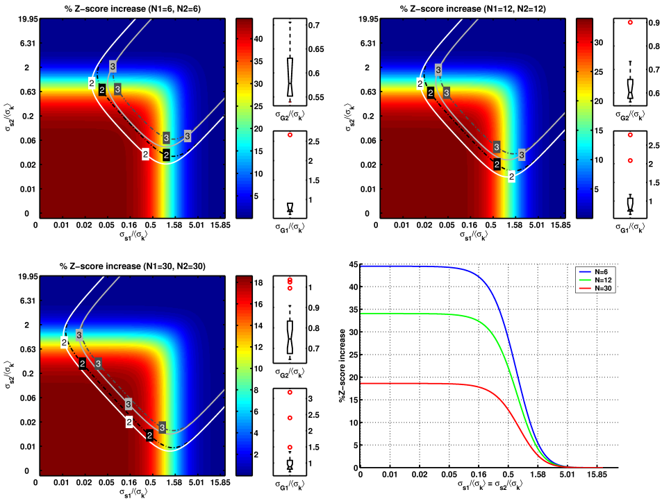
Figure 4 shows numerical simulation of the expected $Z$-score increase for different first-level variance configurations. As before, the expected increase is independent of the second-level effect size but will depend on the first- level variance configuration for group 1 and group 2 as well as the different second-level variances $\sigma_{s1}$ and $\sigma_{s2}$. The added flexibility of the heteroscedastic model is important for a variety of real FMRI experiment where the two groups naturally will have different variance configurations, e.g. studies of patients vs. non-patients. Once again, significant changes in $Z$-score (e.g. $>10\%$) can be seen over a large set of configurations.

Figure: Expected % $Z$-score increase for the unpaired group difference at different group sizes (N=6, 12 and 30). The first three images show the increase as a function of the standard deviation of group 1 and mean first-level standard deviation ( $\sigma_{s1}/ \langle\sigma_{k}\rangle$ on the¥$x$-axis) vs. the standard deviation of group 2 relative to the mean first level standard deviation ( $\sigma_{s2}/ \langle\sigma_{k}\rangle$ on the $y$-axis). Contour lines are shown for the $Z=2.0$ and $Z=3.0$¥ group level thresholds in the case of the heteroscedastic model (solid lines) and homoscedastic model (OLS; dash-dotted). The boxplots show the individual first level standard deviation compared to the mean first-level standard deviation ( $\sigma_{k}/\langle\sigma_{k}\rangle$) as an indicator of heteroscedacity. The expected increase in $Z$- score (assuming $\sigma _{s1}=\sigma _{s2}$) are shown in the fourth plot.