A Simple Partial Volume Model.

Here we take a slightly different approach to modeling in DWMRI. Instead of modeling the diffusion shape directly, we attempt to build a model of the underlying fibre structure which predicts the diffusion shape, and hence the MR measurements. The simplest such model of fibre structure is to assume that all fibers pass through a voxel in the same direction. Assuming no diffusion-diffusion exchange, this leads to a simple two compartment partial volume model. The first compartment models diffusion in and around the axons, with diffusion only in the fibre direction. The second models the diffusion of free water in the voxel as isotropic. One consequence of this model is that the diffusivity (and hence the restriction to water diffusion) in all directions perpendicular to the fibre axis is constrained to be the same. This is very different to the Diffusion Tensor model, where any ellipsoidal diffusion shape may be modeled.

The predicted diffusion signal is

$$\mu_i = S_0((1- f)\exp(-b_id)$$

$$+f\exp(-b_id\vec{r_i}^T\vec{R}\vec{A}\vec{R}^T\vec{r_{i}}))$$ (12)

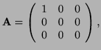
where $d$ is the diffusivity, $b_i$ and $\vec{r_i}$ are the b-value and gradient direction associated with the $i^\textrm{th}$ acquisition, $f$ and $\vec{R}\vec{A}\vec{R}^T$ are the fraction of signal contributed by, and anisotropic diffusion tensor along, the fibre direction $(\theta,\phi)$. That is $\vec{A}$ is fixed as:

$$\vec{A}=\left(\begin{array}{ccc} 1&0&0\\ 0&0&0\\ 0&0&0 \end{array}\right),$$ (13)

and $\vec{R}$ rotates $\vec{A}$ to $(\theta,\phi)$:

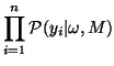
Again noise is modeled as $iid$ Gaussian:

$$\mathcal{P}(\vec{Y}\vert\omega,M) = \prod_{i=1}^n \mathcal{P}(y_i\vert\omega,M)$$

$$\mathcal{P}(y_i\vert\omega,M) \sim \mathcal{N}(\mu_i,\sigma),$$ (14)

where the parameter set $\omega$ now has 6 free parameters ( $\sigma,S_0,d,f,\theta,\phi$). Each of these parameters is subject to a prior distribution, which are chosen to be non-informative except for where we ensure positivity:

$$\mathcal{P}(\theta,\phi)\propto\sin(\theta)$$

$$\mathcal{P}(S_0)\sim\mathcal{U}(0,\infty)$$

$$\mathcal{P}(f)\sim\mathcal{U}(0,1)$$

$$\mathcal{P}(d)\sim\Gamma(a_d,b_d)$$

$$\mathcal{P}(\frac{1}{\sigma^2})\sim\Gamma(a_\sigma,b_\sigma).$$ (15)