Next: Tensor PICA
Up: tr04cb1
Previous: Introduction
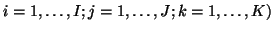
The three-way PARAFAC technique is characterised by the following generative model:
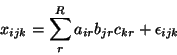 |
(1) |
(
 with an associated
sum-of-squares loss:
with an associated
sum-of-squares loss:
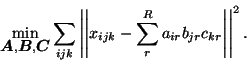 |
(2) |
Here,
 and
and
 denote the
  ,
,  and
and  matrices containing the
  different factor loadings in the temporal, spatial and subject domain
as column vectors. Within this model, any solution to equation 1
different factor loadings in the temporal, spatial and subject domain
as column vectors. Within this model, any solution to equation 1![[*]](icons/crossref.png) is a maximum likelihood solution under the
assumptions of Gaussian noise.
is a maximum likelihood solution under the
assumptions of Gaussian noise.
The tri-linear model can alternatively be written in
matrix notation, giving an expression for the individual 2-D subsets
of
 [Bro, 1998]:
where
 denotes a
  diagonal matrix where the
diagonal elements are taken from the elements
in row
diagonal matrix where the
diagonal elements are taken from the elements
in row  of
of
 (similarly for
 and
and
 ).
This gives rise to a set of coupled sum-of-square
loss functions. Based on these, a simple way of estimating the factor
matrices is to use an iterative Alternating Least Squares (ALS) approach,
iterating between the least-squares estimates for one of
).
This gives rise to a set of coupled sum-of-square
loss functions. Based on these, a simple way of estimating the factor
matrices is to use an iterative Alternating Least Squares (ALS) approach,
iterating between the least-squares estimates for one of
 and
and
 separately while keeping the other two matrices fixed at
their most recent estimate:
separately while keeping the other two matrices fixed at
their most recent estimate:
where  denotes the direct (or element-wise) product. The ALS algorithm
iteratively calculates OLS estimates for the three factor
matrices. Directly fitting these so as to minimise the sum-of-squares error provides a
simple way of jointly estimating the factor loadings that describe
processes in the temporal, spatial and subject domain without
requiring orthogonality between factor loadings in any one of the
domains: the multi-way PARAFAC model, unlike PCA, does not suffer from
rotational indeterminacy, i.e. a rotation of estimated factors has impact
on the overall fit [Harshman and Lundy, 1984,Harshman and Lundy, 1994].
The ALS algorithm , however, can suffer from slow convergence, in
particular, when a set of column vectors in one of the factor matrices
is (close to being) collinear. Also, it is sensitive to specifying the
correct number of factors (i.e. the number of columns in
and
). In order
to address these issues, [Cao et al., 2000] have proposed to extend the
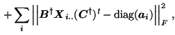
standard PARAFAC loss function to include a diagonalisation error,
such that
denotes the direct (or element-wise) product. The ALS algorithm
iteratively calculates OLS estimates for the three factor
matrices. Directly fitting these so as to minimise the sum-of-squares error provides a
simple way of jointly estimating the factor loadings that describe
processes in the temporal, spatial and subject domain without
requiring orthogonality between factor loadings in any one of the
domains: the multi-way PARAFAC model, unlike PCA, does not suffer from
rotational indeterminacy, i.e. a rotation of estimated factors has impact
on the overall fit [Harshman and Lundy, 1984,Harshman and Lundy, 1994].
The ALS algorithm , however, can suffer from slow convergence, in
particular, when a set of column vectors in one of the factor matrices
is (close to being) collinear. Also, it is sensitive to specifying the
correct number of factors (i.e. the number of columns in
and
). In order
to address these issues, [Cao et al., 2000] have proposed to extend the
standard PARAFAC loss function to include a diagonalisation error,
such that
(similarly for
 and
and
 ). Here,
 denotes the Fröbenius norm and
 denotes the pseudo-inverse of
 . The first
term corresponds to the sum-of-square loss function while the second
term penalises the
. The first
term corresponds to the sum-of-square loss function while the second
term penalises the  different projection
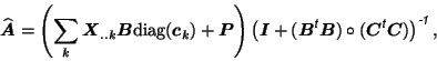
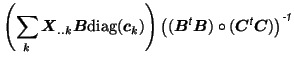
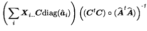
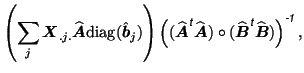
matrices. A modified ALS algorithm can be derived
by iterating solutions for
different projection
matrices. A modified ALS algorithm can be derived
by iterating solutions for
with
 . The ordinary least-squares solutions then
becomes [Cao et al., 2000]:
. The ordinary least-squares solutions then
becomes [Cao et al., 2000]:
where
![$\mbox{\protect\boldmath$P$}=[\mbox{\protect\boldmath$p$}_1,\dots,\mbox{\protect\boldmath$p$}_I]^{\mbox{\scriptsize\textit{\sffamily {t}}}}$](img51.png) and where
and where
 are column
vectors formed by the elements on the main diagonal of the
matrix
are column
vectors formed by the elements on the main diagonal of the
matrix
 (similar for
 and
and
 ). This modified ALS algorithm has been used for all later PARAFAC
calculation.
). This modified ALS algorithm has been used for all later PARAFAC
calculation.
It is interesting to note that the ALS approach to three-way PARAFAC does
provide a unique decomposition, provided the data has appropriate
'system variation' [Harshman and Lundy, 1984,Harshman and Lundy, 1994], i.e. when
and
are of full rank and there are
proportional changes in the relative contribution from one factor to
another in all three domains so that no two factors in any
domain are collinear. In FMRI, however, we might expect the
individual vectors in subject space to exhibit a significant amount
of collinearity between some of them, e.g. in the case of two
spatially different physiological signals, we might expect the
relative contribution of the individual subjects to be very similar,
so that two columns in
are (close to being) collinear. The
effects of collinearity of some of the factors on the ability to
extract the latent structure of the data will be evaluated in section 4.
Next: Tensor PICA
Up: tr04cb1
Previous: Introduction
Christian Beckmann
2004-12-14