MRF precision updates

Here we give the update equation for the MRF precision parameter distribution $q(\phi_{a_p}\vert y)=Ga(b_{\phi_{a_p}},c_{\phi_{a_p}})$:

$$\frac{1}{b_{a_p}} = \frac{1}{2}\left(m_{a_p}^TD m_{a_p} + \text{Trace}(\Lambda_{a_p}D)\right)+\frac{1}{b_{a_0}}$$ (43)

$$c_{a_p} = N/2+c_{a_0}$$ (44)

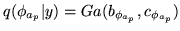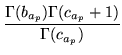
we define $\gamma_{a_p}$ as:

$$\gamma_{a_p} = \frac{\Gamma(b_{a_p})\Gamma(c_{a_p}+1)}{\Gamma(c_{a_p})}$$ (45)

Even though the matrix $D$ is very sparse the computation of the Trace$(\Lambda_{a_p}D)$ term can be very expensive to compute. In particular, this is because $\Lambda_{a_p}=F_{a_p}^{-1}$ and $F_{a_p}$ is a $N\times N$ matrix whose inverse would be very computationally expensive to compute. Therefore, instead of computing this inverse we can compute $x$ in the linear equation:

$$F_{a_p}x = D$$ (46)

Since $D$ is a positive symmetric definite matrix we can take advantage of the conjugate gradient techniques described in Golub and Van Loan (1996). At each iteration of the conjugate gradient search for $x$ we only need to perform one matrix multiplication of $F_{a_p}x$. The conjugate gradient approach is far quicker than solving for the inverse of $F_{a_p}$ and then multiplying by $D$.

The conjugate gradient technique takes in an initial guess of $x$. Hence, as we iterate through the Variational Bayes updates of our approximate posterior distributions, we can store the the value of $x$ from the previous conjugate gradient solution from the previous update of $q(\phi_{a_p}\vert y)$, and use it as the initialisation of the conjugate gradient search for $x$ at the next update of $q(\phi_{a_p}\vert y)$. After the first Variational Bayes iteration this makes subsequent conjugate gradient searches very quick to converge.