Example Box: Independent Component Classification
Introduction
The aim of this example is to become familiar with what resting state fMRI data looks like and what can be found using independent component analysis (ICA).
This example is based on tools available in FSL, and the file names and instructions are specific to FSL. However, similar analyses can be performed using other neuroimaging software packages.
Please download the dataset for this example here:
Data download
The dataset you downloaded contains the following files:
- Pre-processed resting state fMRI images:
filtered_func_data.nii.gz - A directory containing the results of an ICA analysis:
filtered_func_data.ica - A text file providing labels for the ICA components:
labels.txt
Viewing the Data
To start with load the fMRI data filtered_func_data.nii.gz into a viewer (e.g. fsleyes) and inspect the image. You will see that there are many time points, each of which looks visually very similar as the fMRI signals of interest cannot be seen by eye (as they are on the order of 1% of the mean intensity). These images have already been motion corrected and filtered, but the appearance is very similar to the original data.
Close this viewer as we will start a new one that is setup to display the ICA results. To do this open a terminal and change directory (with cd) to the directory with this data. Then do:
fsleyes --scene melodic -ad filtered_func_data.ica &
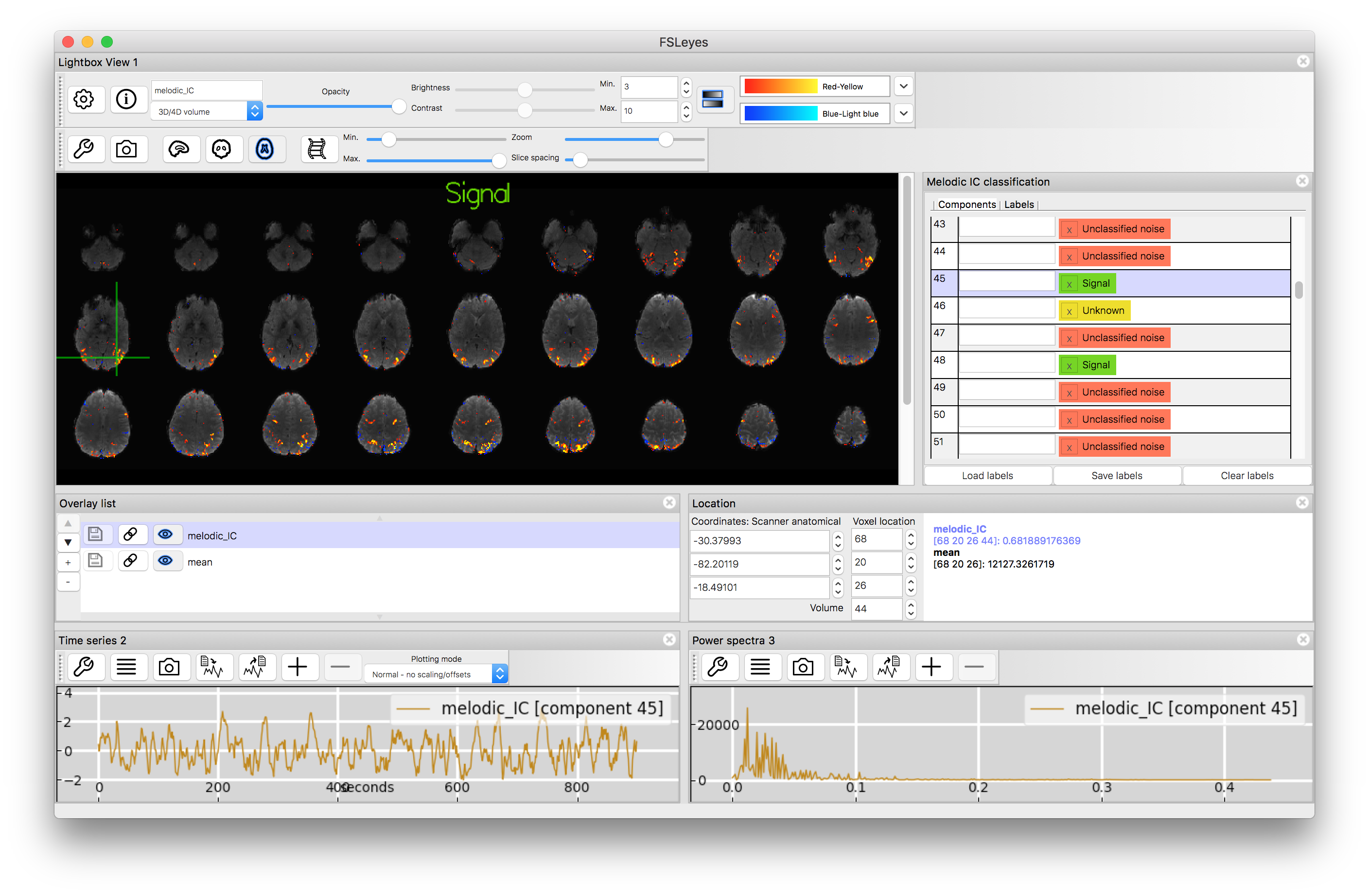
which will open a window that shows the ICA result (coloured) on top of the brain (in grey) along with the timeseries and the frequency spectrum of the component (at the bottom). Note that the same thing can be achieved through the GUI alone, using View --> Perspectives --> MELODIC mode. In other viewers the main data file to be loaded is melodic_IC.nii.gz which contains the spatial maps, with other text files containing information about the timecourses and frequency spectra.
Flick through some different components by highlighting the "melodic_IC" in the Overlay list and then changing the "Volume" number. You will see a range of very different spatial maps, timecourses and frequency spectra. Try adjusting the "slice spacing" and surrounding controls so that you can see a good range of slices, covering most of the brain.
The list of labels in the right hand window "Melodic IC classification" is currently at the default (all "unknown") so now load the manual labels from the label.txt file. Do this by using the "Load labels" button underneath the label list and then finding the label.txt file. This may give you a warning message about the location changing, in which case just select the option to "Apply" the labels to the current data. Once you have done this you will see that each component has a label. Scroll through this to find a "signal" component and then click on it to display that component.
You will find that the signal components are not only more biologically interpretable with respect to the spatial map but they have frequency spectra that are dominated by lower frequencies and, typically, timecourses that look "sensible" (i.e. without major spikes or steps or other odd features). Some of the noise components will share some of these features, but not all. Classifying ICA components is a skill that requires some experience, as not all components are obvious, and you will find several components classified as "unknown" in the list.
The labels here are useful for inspecting this data but are also used for training an automatic classifier, where the main objective is to remove components that are clearly noise and leave behind others (signal or unknown) in order to get cleaner data.
This example should give you some experience at looking at ICA results for resting state data. Take your time and look through many components (though no need to do them all) in order to get a feeling for the different types of signal, noise and artifacts - as also shown in the Primer text.