Example Box: Task fMRI Data

Introduction

The aim of this example is to become more familiar with task fMRI data, the results of the analysis and how they can be affected by pre-processing choices.

This example is based on tools available in FSL, and the file names and instructions are specific to FSL. However, similar analyses can be performed using other neuroimaging software packages.

Please download the dataset for this example here:

Data download

The dataset you downloaded contains the following files:

Original fMRI data: fmri.nii.gz
Structural data (original and brain extracted): structural.nii.gz and structural_brain.nii.gz
Timing files describing the stimuli: word_shadowing.txt, word_generation.txt and null_events.txt
A directory containing pre-calculated analysis results: fmri.feat

where the analysis has been done using the FSL tool FEAT.

The Experiment

Before looking at the data we will describe the experiment. This dataset fmri.nii.gz is from an event-related language experiment and has three different types of events:

Word-generation events (WG): Here the subject is presented with a noun, say for example "car" and his/her task is to come up with a pertinent verb (for example "drive") and then "think that word in his/her head". The subject was explicitly instructed never to say or even mouth a word to prevent movement artefacts.
Word-shadowing events (WS): Here the subject is presented with a verb and is instructed to simply "think that word in his/her head".
Null-events (N): These are events where nothing happens, i.e. the cross-hair remains on the screen and no word is presented. The purpose of these "events" is to supply a baseline against which the other two event types can be compared.

Note that there were no additional "instruction events" as part of the experiment. Each event was "its own instruction" in that the class of the word determines the task. This means that even the "shallow" word-shadowing events contain an element of grammatical decoding.

Within one session, the events were presented at a constant ISI (Inter Stimulus Interval) of 6 seconds. For example, the first 72 seconds (twelve events) in this session may have looked like:

N-WS-N-WS-N-WS-N-WG-N-WS-WG-N

The randomisation of event types was "restricted" in the sense that there was an equal number (24) of each event type. In other words, at any given ISI each type of event was equally likely.

The main question for this experiment was to see if the "deeper" language processing in the word-generation task would yield activations over and above that of the shallower processing in the word-shadowing task. But there are also other interesting questions you can ask of the data.

Viewing the Data

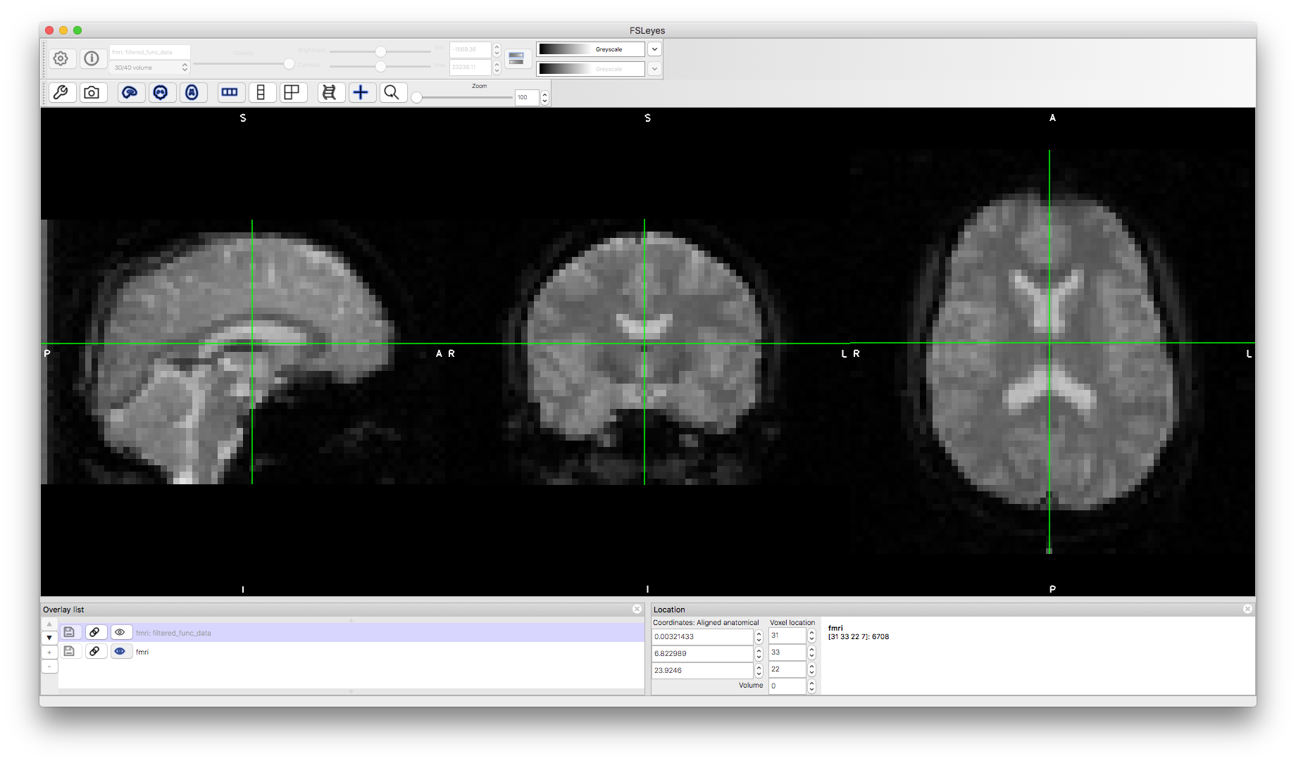
To start with load the original data fmri.nii.gz into a viewer (e.g. fsleyes). Note that the data has fairly low resolution (voxel size of 3.5mm isotropic and the TR is 4.2 seconds). If you change the "Volume" number or turn the movie mode on then you will see some changes (particularly near the brainstem) but no obvious head movements or areas of activation. This is because the physiological effects (e.g., pulsatility) are much more obvious, while the size of motion-induced changes are much less (for cooperative subjects like this that stay still) and activation changes are even less (only about 1% change compared to the mean intensity). Areas of geometric distortion and signal loss are also present in these scans, though with this low resolution it is difficult to easily see them.

Pre-Processed Data

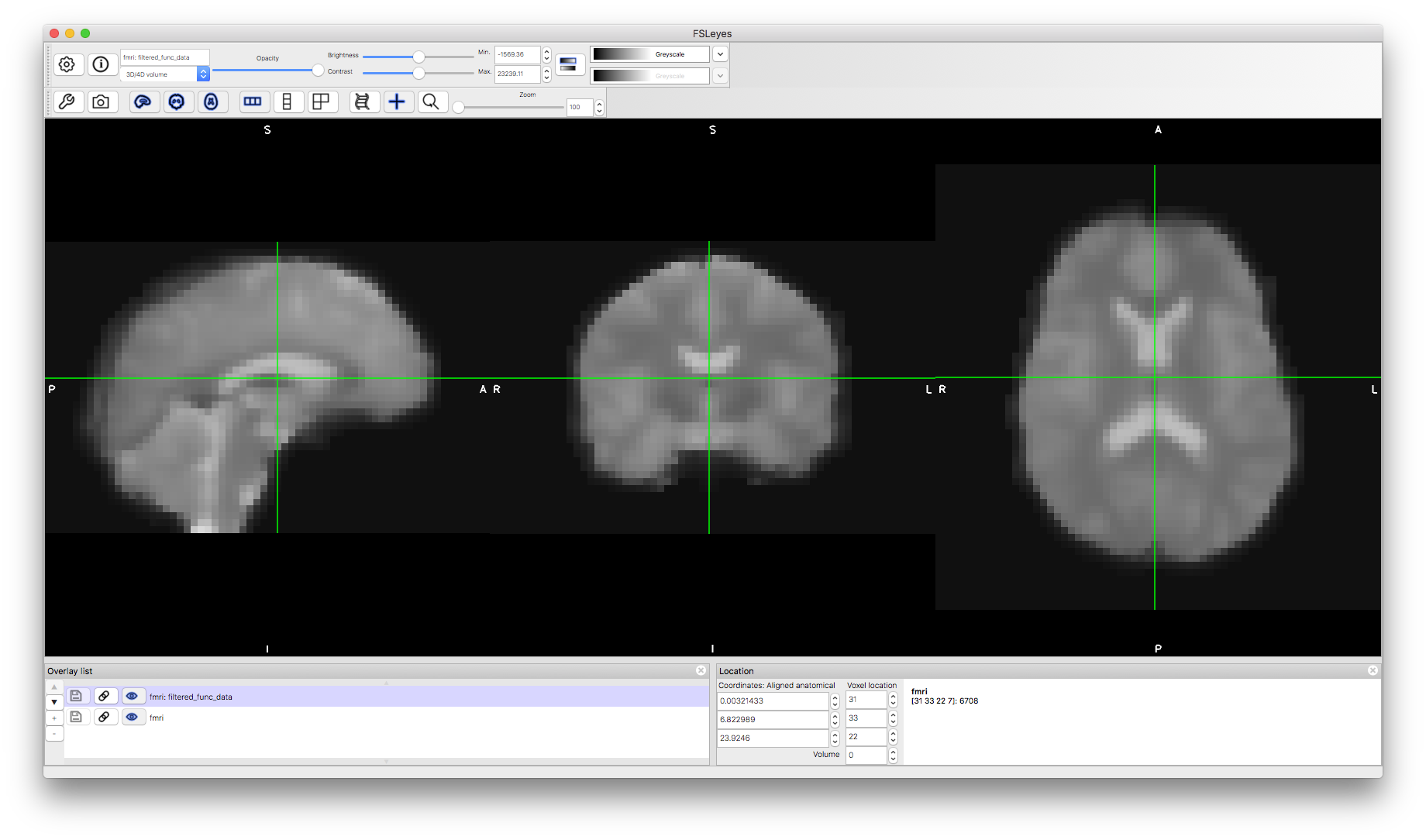
Now let's look add the pre-processed data to the viewer. You can find this in the results directory fmri.feat and it is called filtered_func_data.nii.gz. The immediately obvious thing about this is how much smoother it is, due to the spatial filtering that was applied.

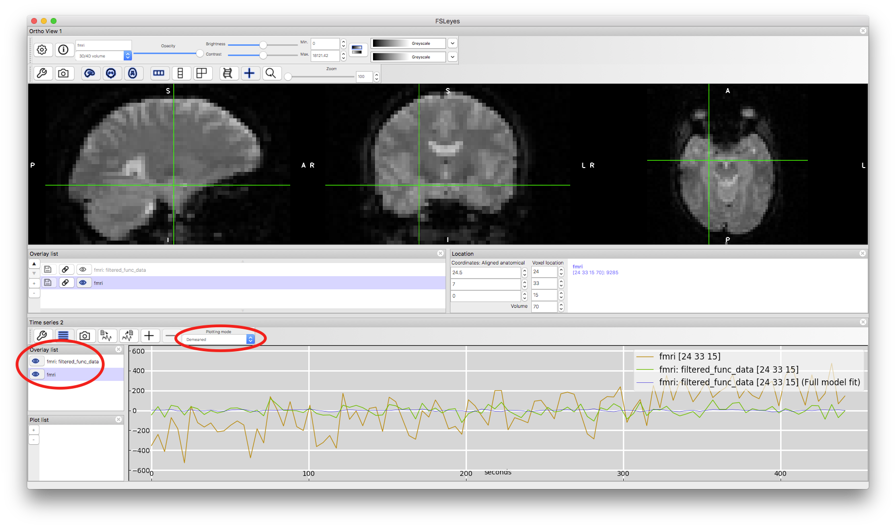
We can also examine the effects of the highpass temporal filter. To do this we will turn on the "Time series" view (from the View menu in fsleyes). This will show the timeseries in the different images here as well as the final model fit (as it reads this automatically from the results directory). To see both timeseries clearly at the same time you need to select the "Demeaned" option from the "Plotting mode" pull-down menu, as otherwise the arbitrary mean value (which is modified in the pre-processing) dominates the difference and makes it hard to see the changes in time. When you have done this make sure that both the fmri and filtered_func_data images are highlighted in the Overlay list for the timeseries window (to the left of the timeseries). This will then show you the original data (from fmri) and the pre-processed data (from filtered_func_data) from the voxel that your crosshairs are on. Click around some other voxels in the image window and see the timeseries change. Most of them do not contain any sizeable drift but some do, and there the effect of the filtering is most obvious (e.g., voxel coordinate 24,33,15 starts low and drifts upwards throughout - you should be able to find other examples too). Note that the size of the intensity changes is also scaled in the pre-processing, but this is not a cause for concern as the analysis is insensitive to scaling (as it scales both the signals of interest and the noise equally).

Analysis Results

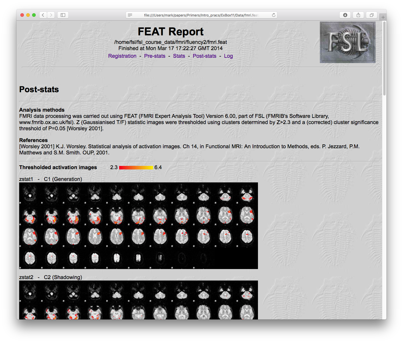
The results of an analysis with the tool FEAT can be found in fmri.feat and the most convenient way to get an overview of them is to load the webpage report: report.html. Open this in a web browser and then click on the "Post-stats" link near the top. This will show a page with a number of statistical result images and some timeseries plots underneath. Each image corresponds to the results from a contrast that was specified in the analysis (shown along with the names given to them by the experimenter). These contrasts are how specific hypothesis (questions) are formulated and tested. For instance, in this analysis there were five contrasts:

Generation: this tests for when there was greater activation during word generation compared to baseline.
Shadowing: this tests for when there was greater activation during word shadowing compared to baseline.
Mean: this tests for when the average activation during generation and shadowing was greater than baseline.
Shad > Gen: this tests for when there was greater activation during word shadowing compared to word generation.
Gen > Shad: this tests for when there was greater activation during word generation compared to word shadowing.

Each image shows voxels (in colour) that are statistically significant for that particular hypothesis, or contrast. All the results are corrected for multiple comparisons. The timeseries below show what the timeseries and model fits look like for the single strongest voxel in each contrast - these are normally of limited interest, so we won't go into details of them here.

It is also possible to load the statistical results into a viewer and interact with them more fully in 3D. There are two statistical results saved that are most useful: thresholded and unthresholded. The thresholded results are in the directory fmri.feat and are named thresh_zstat1.nii.gz and so on (the number is the number of the corresponding contrast). The unthresholded statistical values are stored in a subdirectory fmri.feat/stats/ and are named zstat1.nii.gz and so on.

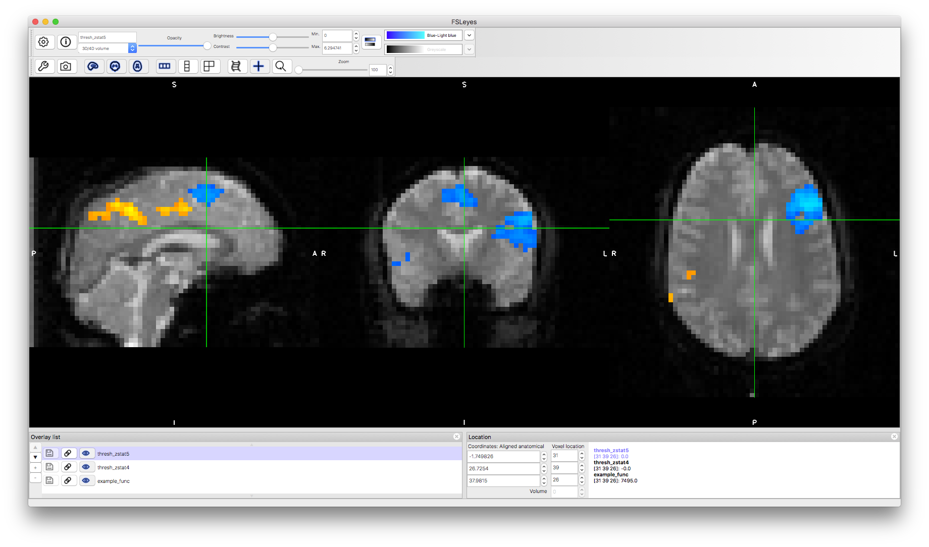
To load these into a viewer it is helpful to start by loading an example functional image, to see the brain anatomy. Open the image fmri.feat/example_func.nii.gz in the viewer and then add both fmri.feat/thresh_zstat4.nii.gz and fmri.feat/thresh_zstat5.nii.gz. Apply different colourmaps to the latter two images, as this makes it easier to view both results simultaneously (these results are for "Shad > Gen" and "Gen > Shad" respectively). This is generally the best way to view your results, to identify the anatomical locations, and to see how the statistically significant results differ between contrasts.

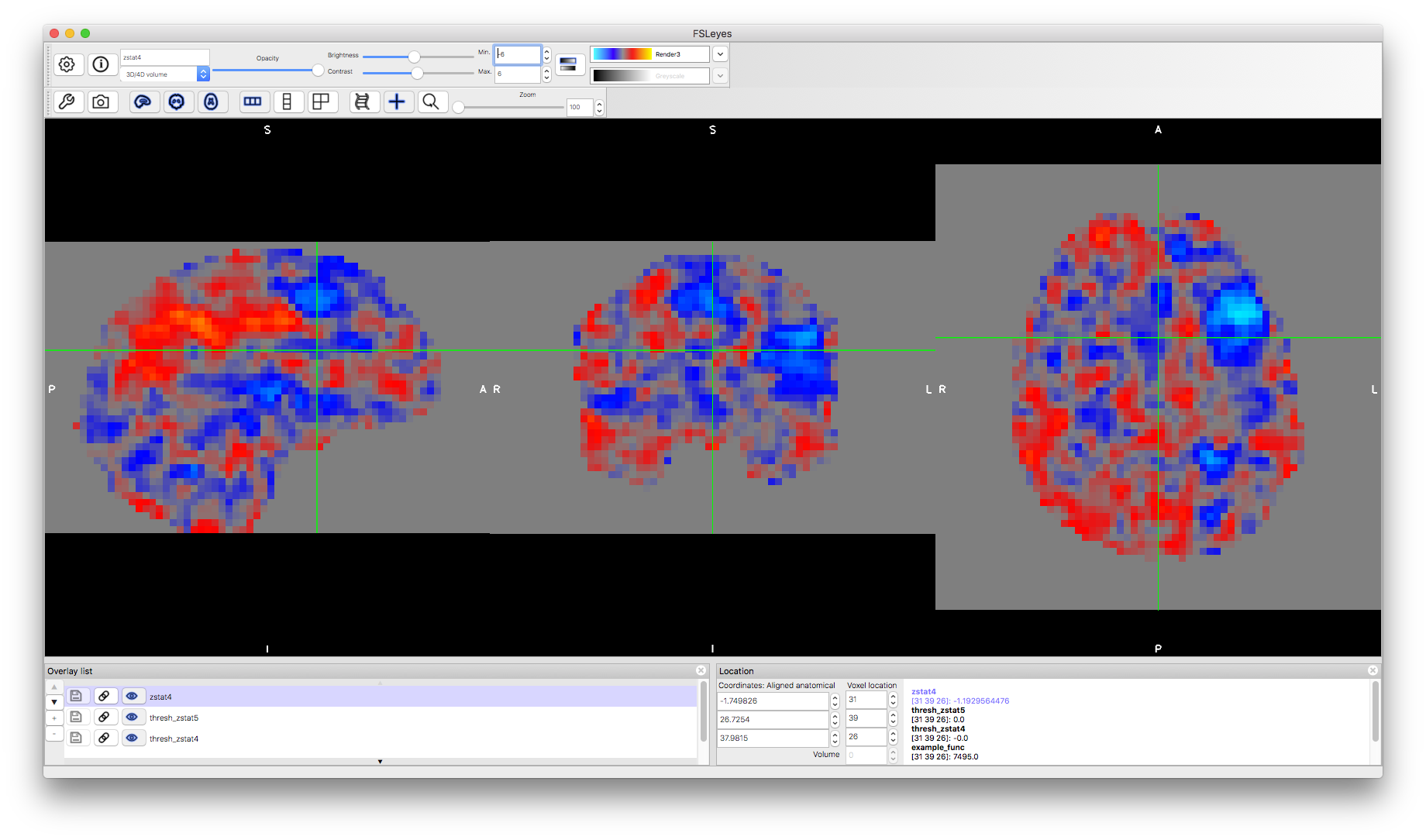
Now load an unthresholded version of the "Shad > Gen" statistics by adding the image fmri.feat/stats/zstat4.nii.gz. You will notice how this covers all the brain, as it shows both positive and negative results, regardless of if they are statistically significant or not (since no threshold has been applied). Change the colormap to "Render3" and set the "Min" to -6 and the "Max" to +6. This will then show you positive statistical values in redder colours and negative values in bluer colours. Although you cannot report anything from these images as being statistically significant, it can be useful to see what is contained in your data and what might be just under a significant threshold, which might become significant in group analyses with more subjects. In this case we are looking at the results from a single subject, but all of these results are also available for group analyses.

Analysis Settings

Finally, we shall look at how the analysis is performed and explore the options available. We can load the full details of this analysis (or any FEAT analysis) into the FEAT GUI. To do this, start the main fsl gui fsl & and then select the FEAT button. This will start the FEAT GUI in a separate window and in that window select the "Load" button and then navigate to the fmri.feat directory and inside that select the file design.fsf. This file contains all the settings that are needed to repeat the analysis. When you load this it will change various values throughout the GUI, which we will explore now.

Go to the "Pre-stats" tab and you will see the various pre-processing settings: e.g., motion correction is "on" and uses the MCFLIRT tool, no "B0 unwarping" is done in this case, no "Slice timing correction" is done here - though it is accounted for in the model - and the "Spatial smoothing FWHM (mm)" is set to 7.0mm. That shows what was used for this specific analysis.

Now go to the "Stats" tab and click on "Full model setup". This brings up a window where the different EVs (or regressors) in the model are specified: in this case two of them - one for word generation and the other for word shadowing (as the null events are the implicit baseline and do not need to be specified separately). There is also a "Contrast and F-tests" tab here where the different contrasts are specified (the five that we listed earlier) and this is also where they are, optionally, given names.

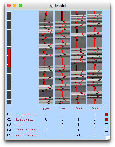
Since this data has been packaged up and moved from the original location, none of the input files can be currently found. However, you can easily reset them to the right locations on your machine. To do this let's start by resetting the files that are used to specify the EV timings. Go to the "EV" tab in the last window we looked at and click on the file browser for the "Filename" and then find and select the file word_generation.txt. Do the same for the second EV (select tab "2" for the settings) by use the file word_shadowing.txt. Once you've reset both of these then click on "View design" at the bottom of this window and you should see the GLM design matrix (as shown below) where you have the two EVs associated with the timings that are specified here along with their temporal derivatives (used to account for slice timing changes and additional HRF variations), making 4 EVs in total. It also shows the contrasts underneath. If you get an error then you probably have not specified one or more of the file correctly. Start afresh (open a new instance of the FEAT GUI and load the design.fsf file again) if you think you have done it right but are still getting errors.

You can use this GUI to re-run the analysis and modify some of the settings to see the effect. For instance, try changing the amount of smoothing. In order to run again you must reset all the filenames (not just the two EV timing files that we did above). The full list of files that need to be reset (using the file browser icon in each case) is:

fmri.nii.gz on the "Data" tab - by clicking on the "Select 4D data" button
structural_brain.nii.gz on the "Registration" tab under "Main structural image"
MNI152_T1_2mm_brain.nii.gz on the "Registration" tab under "Standard space".
- Note that this may already be correct if your FSL is installed in /usr/local/fsl but if not then you need to navigate to wherever your FSL is installed and then go into the data/standard directory. Use the "Add standard" button in fsleyes and then inspect the filename with the "(i)" information button if you are unsure where to find these files.

You can leave the "Output directory" blank on the "Data" tab or specify your own output name and location (use the file browser here and whenever it is present, as it minimises the changes of things being put in the wrong place). If you do not specify an output directory name then FEAT will take the name of the input 4D data file and replace .nii.gz with .feat as had already been done here. If that .feat directory already exists then it will create a new one using a "+" sign, or "++" if there was already a "+", etc. For instance, if you re-ran this analysis now you would create a directory called fmri+.feat

If you have time, try re-running this analysis with some different settings and see what happens. It should load a webpage that gives you a report on progress, but if not just look for the output files. An analysis typically takes anywhere from 5 to 30 minutes.

This example should give you practical experience looking at fMRI data, results from the analysis, as well as information on how to run such an analysis with the FSL tools. The dataset is also part of an FSL Course practical, so if you would like more detailed instructions on how to run the analysis on this data please go to the first fMRI practical on the FSL Course as well as the FEAT page on the FSL wiki.