Example Box: Registration Case Studies
Introduction
The aim of this example is to become familiar with the data and the steps involved in doing the registrations depicted in the three case studies in section 5.4 of the Introduction to Neuroimaging Analysis Primer.
This example is based on tools available in FSL, and the file names and instructions are specific to FSL. However, similar analyses can be performed using other neuroimaging software packages.
Please download the dataset for this example here:
Data download
The dataset you downloaded contains the following:
- Original (non-brain-extracted) T1-weighted image:
T1.nii.gz - Original (non-brain-extracted) T2-weighted image:
T2.nii.gz - A single 3D volume from a functional acquisition:
func.nii.gz - A fieldmap acquisition (phase and magnitude):
fmap_phase.nii.gzandfmap_mag.nii.gz - A white matter segmentation (calculated using the T1-weighted structural):
T1_wmseg.nii.gz - Directory containing previously generated results:
pre_baked
Case 1: Two structural images of the same subject
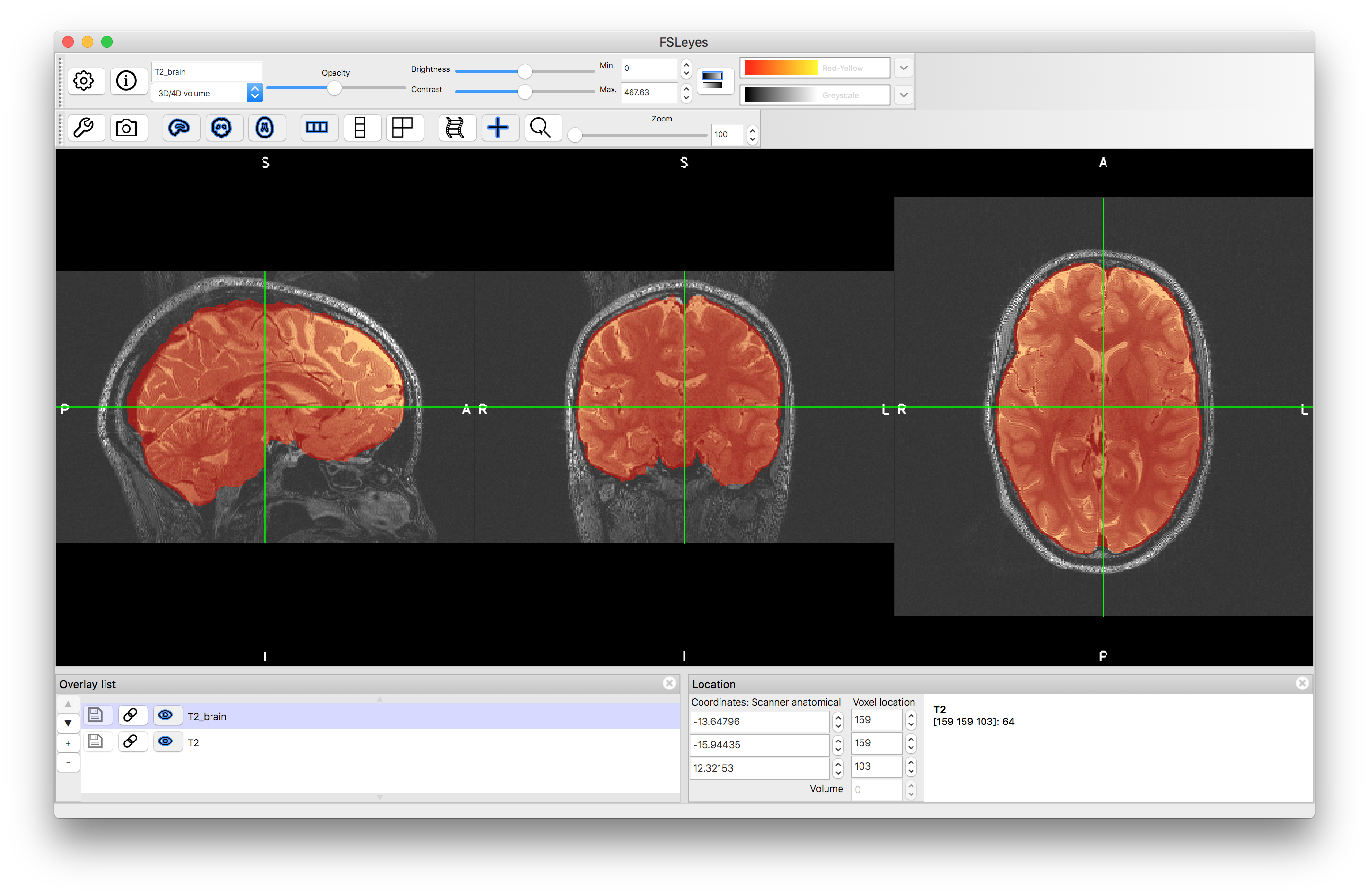
To start with load both the original images (T1.nii.gz and T2.nii.gz) into a viewer (e.g. fsleyes) and inspect them. Note that they are quite high resolution (0.8mm) but not well aligned to start with.
The first step for registration of these images is to perform brain extraction. This can be done (in a terminal) with the two commands below:
bet T1.nii.gz T1_brain.nii.gz
bet T2.nii.gz T2_brain.nii.gz -f 0.2
Load the results (T1_brain.nii.gz and T2_brain.nii.gz) into a viewer and visually assess the accuracy. Note that in the second brain extraction the "fractional intensity threshold" was lowered to 0.2 to get a good result. Try it with the default value (-f 0.5, which is what you get if you omit the -f option entirely) and see what the result looks like. There should be obvious areas of missing brain tissue in the inferior regions.
Now that we have two brain extracted images we will perform a 6 DOF registration, initially using the Correlation Ratio as the cost function. This is because we need a cost function that is suitable for different modalities, which rules out Least Squares and Normalised Correlation. The FSL tool for linear registration, FLIRT, can be run with the following command:
flirt -in T2_brain.nii.gz -ref T1_brain.nii.gz -dof 6 -cost corratio -omat T2toT1_cr.mat -out T2toT1_cr.nii.gz
Load the result T2toT1_cr.nii.gz into a viewer and compare it with the reference image T1_brain.nii.gz. As shown in Figure 5.8, it is very helpful to overlay red edges from the T1-weighted image that correspond to the white matter boundary. In the pre_baked directory you can find an image containing these edges called func2struct_fast_wmedge.nii.gz (it will be generated during one of the later calls) and you can load this and give it a ref colourmap to see the same display as in the image below and in Figure 5.8. You can also easily generate the edge image from the white matter segmentation (T1_wmseg.nii.gz) with a single command. We will describe how to get the segmentation itself below.
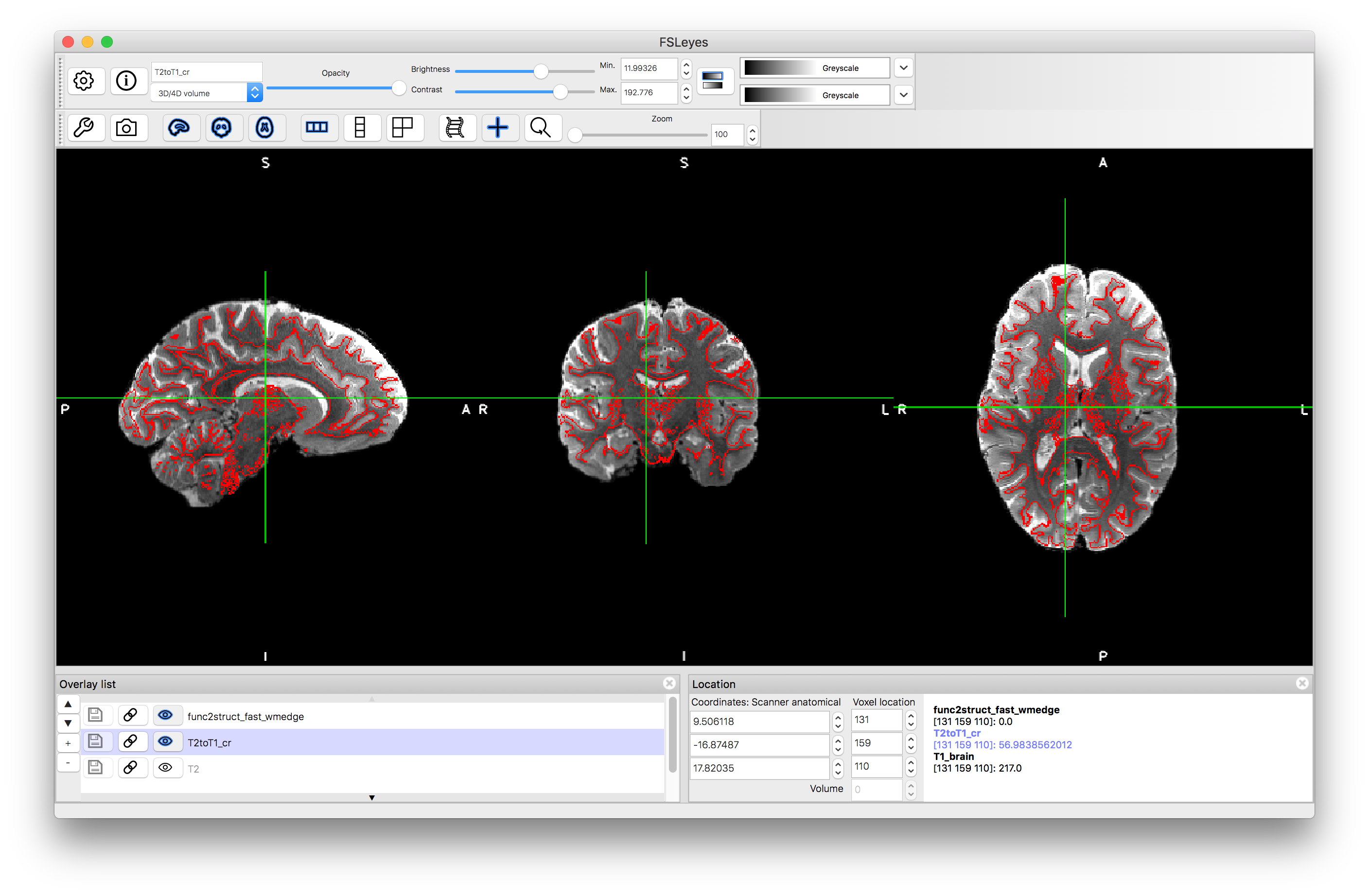
Also view the original T2-weighted image with this edge overlay to see how much the registration has improved the alignment. Note that when if you load in a new image you will need to reorder the Overlay List to make sure that the WM edge image is on top of the overlay list in order to see the red edges.
BBR Registration
We will now do the registration again using BBR, to demonstrate how to use this cost function for registration of structural images (it is a little different for functional images - see below). The BBR registration requires initialisation, so we will use the result from the Correlation Ratio registration above. It also requires the white matter segmentation, as internally it will calculate the cost function only around the white matter boundary. The command to do this in FSL is:
flirt -in T2.nii.gz -ref T1_brain.nii.gz -dof 6 -cost bbr -wmseg T1_wmseg.nii.gz -schedule $FSLDIR/etc/flirtsch/bbr.sch -init T2toT1_cr.mat -omat T2toT1_bbr.mat -out T2toT1_bbr.nii.gz
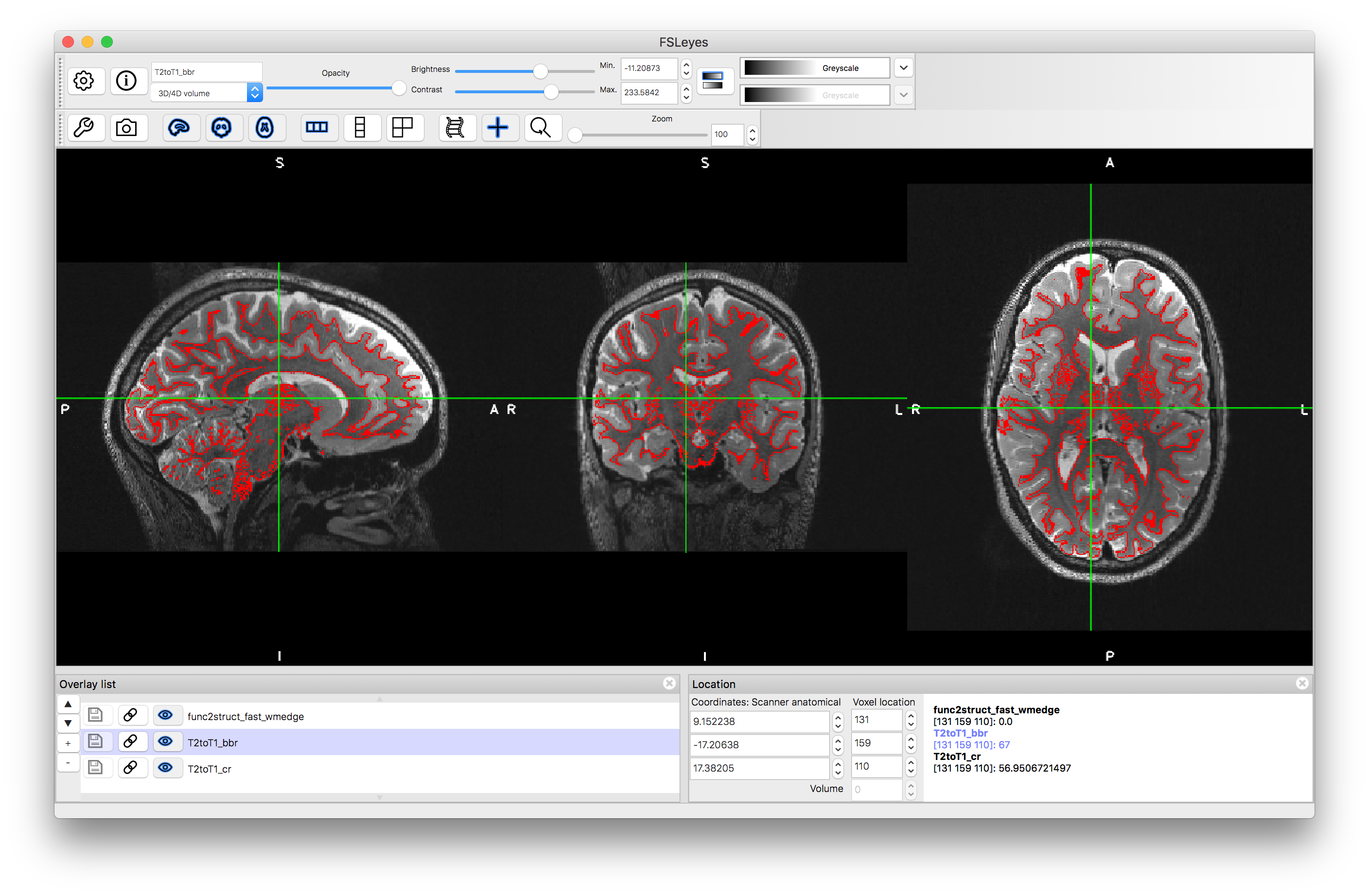
Here we use the non-brain-extracted T2-weighted image, although it would make little difference if we used the brain extracted version (since all the calculation is around the white matter boundary). We also use the T2toT1_cr.mat (the output spatial transformation - in matrix form - of the Correlation Ratio registration) to initialise. Once you have run this command (which could take 5-20 minutes to run) load the output T2toT1_bbr.nii.gz into your viewer along with the previous results and see whether you prefer the BBR result or the Correlation Ratio result (Figure 5.8 shows the key areas to inspect - e.g. boundaries in the occipital, parietal and cerebellar areas near the midline, and around the anterior ventricles).
Case 2: Structural image of one subject and the MNI152 template
To register the T1-weighted image to the MNI152 template we will follow the same procedure as described in the previous example box. This involves an initial affine (12 DOF) registration to the MNI152 template followed by a nonlinear registration. The commands for this are:
flirt -in T1_brain.nii.gz -ref $FSLDIR/data/standard/MNI152_T1_2mm_brain.nii.gz -dof 12 -out T1toMNIlin.nii.gz -omat T1toMNIlin.mat
fnirt --in=T1.nii.gz --aff=T1toMNIlin.mat --config=T1_2_MNI152_2mm.cnf --iout=T1toMNInonlin.nii.gz --cout=T1toMNI_coef.nii.gz --fout=T1toMNI_warp.nii.gz
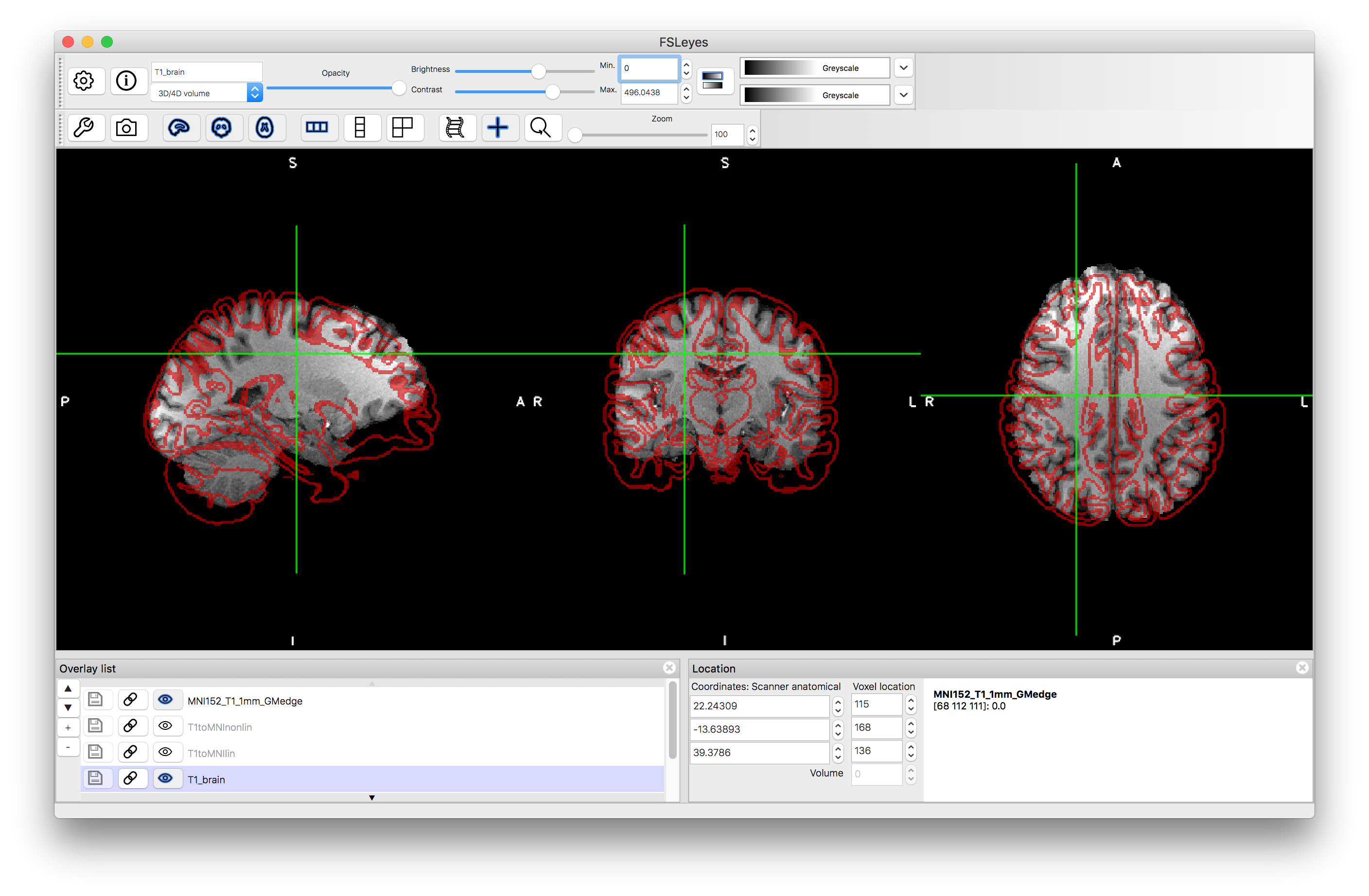
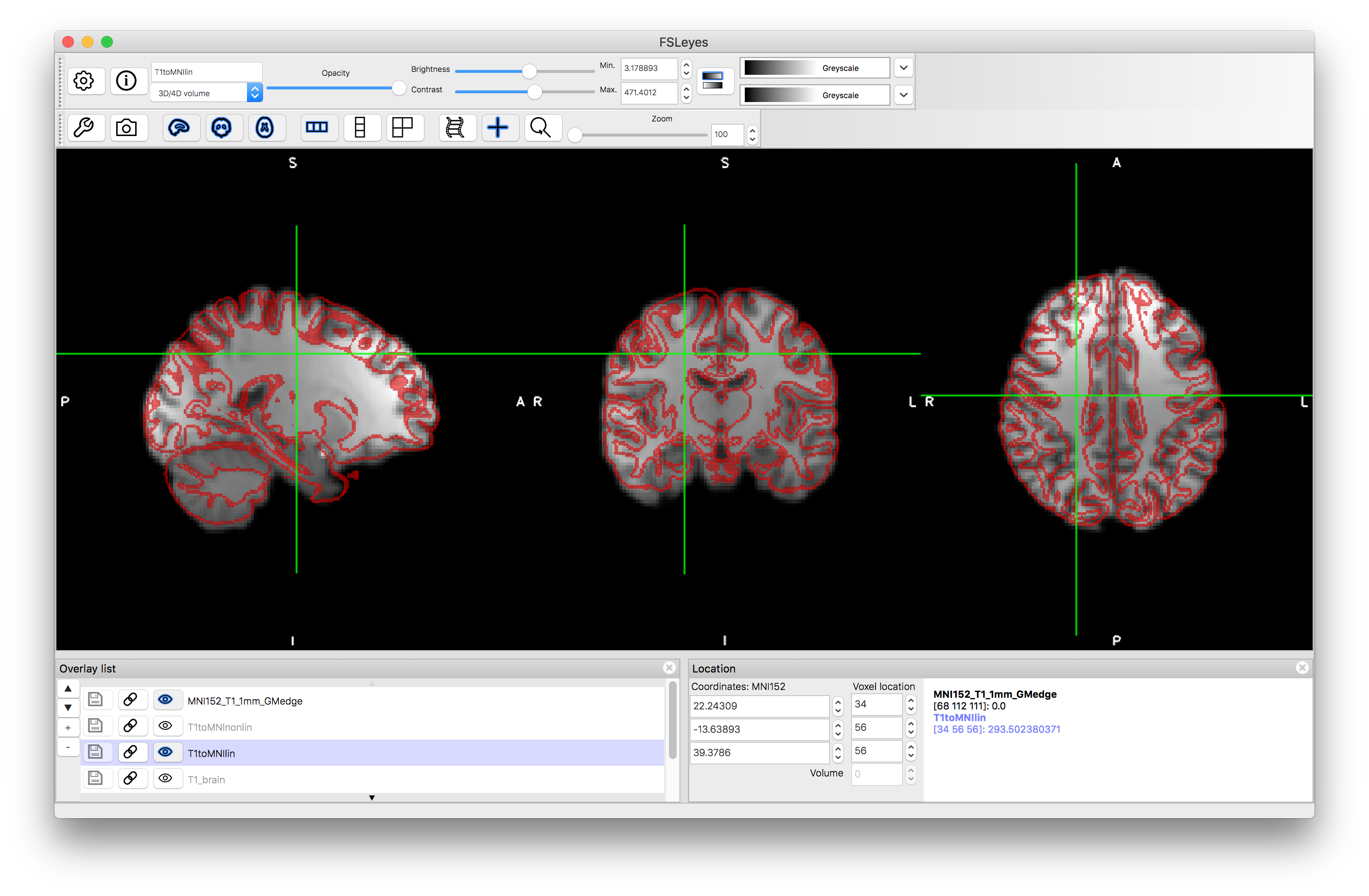
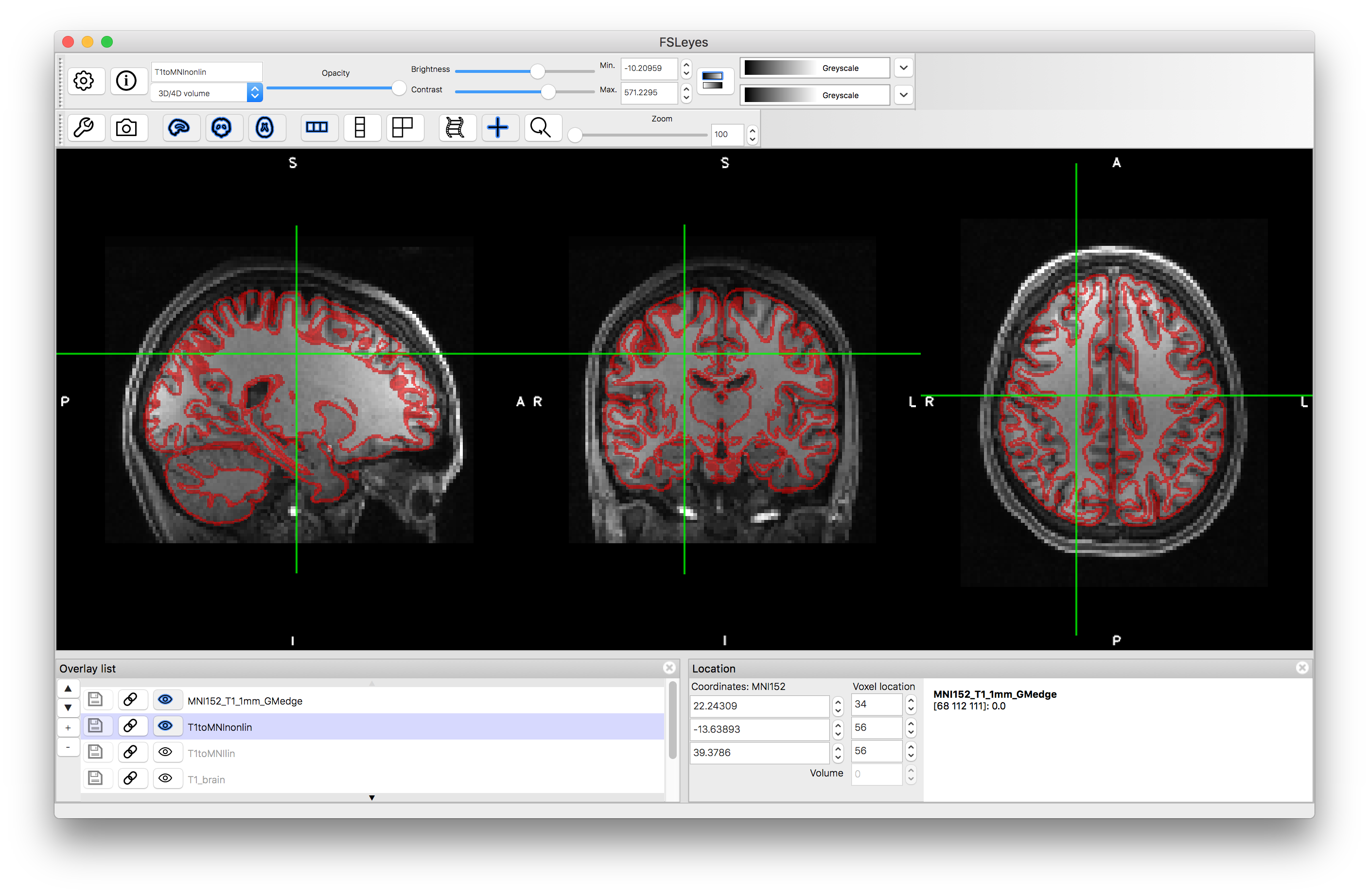
Load the outputs T1toMNIlin.nii.gz and T1toMNInonlin.nii.gz along with T1-brain.nii.gz and overlay red edges (gray matter boundaries in this case) from the MNI152 (pre_baked/MNI152_T1_1mm_GMedge.nii.gz) into a viewer. Compare the accuracy of the alignment in each case, although remember that it is normal that smaller folds are less accurately aligned, even with the nonlinear registration (due to variation in the population, as reflected in the MNI152 template). Also load the standard template (MNI152_T1_1mm.nii.gz) to compare directly to this.
Linear registration:
Nonlinear registration:
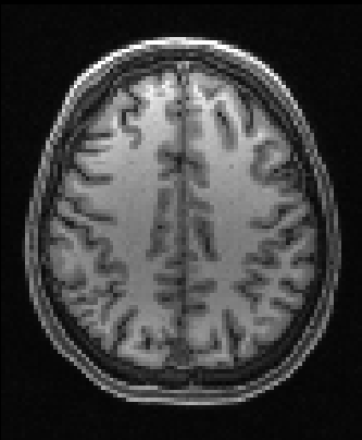
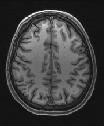
One thing that you will have seen from these results is that they are low resolution (2mm), which is due to using the 2mm MNI152 template for the registration. This is sufficient for calculating the registration to this template (since the details in the MNI152 template are often somewhat blurry due to population variations) but it is often desirable to produce a sharper result with better resolution. This can easily be done by applying the transformation (that is calculated in the registration step) to the original image again, but with a better reference/output resolution and different interpolation. To do this in FSL the command is:
applywarp -i T1.nii.gz -r $FSLDIR/data/standard/MNI152_T1_1mm.nii.gz -w T1toMNI_warp.nii.gz --interp=spline -o T1toMNInonlin_1mm.nii.gz
Load this result into a viewer to see the difference between this and the previous output.
| Nonlinear registration output | ||
| 2mm resolution | 1mm resolution | |
 |
 |
|
All of the above steps can also be repeated for other datasets - such as those shown in Figure 5.9, and you can find some data for this in one of the previous example boxes.
Case 3: EPI image (fMRI or dMRI) and structural of one subject and the MNI152 template
Registration of an EPI image to the structural benefits substantially from using fieldmaps to correct the geometric distortion. We will demonstrate how to do this registration using fieldmaps (from a gradient-echo sequence) and the BBR cost function. After this we will combine it with the registration to the MNI standard space, as calculated in Case 2 above.
Fieldmap preparation
The first step is to process the raw fieldmap images to get them into the required form for subsequent registration. This can be done in FSL with the following commands:
bet fmap_mag.nii.gz fmap_mag_brain1.nii.gz
fslmaths fmap_mag_brain1.nii.gz -ero fmap_mag_brain.nii.gz
fsl_prepare_fieldmap SIEMENS fmap_phase.nii.gz fmap_mag_brain.nii.gz fmap_rads.nii.gz 2.46
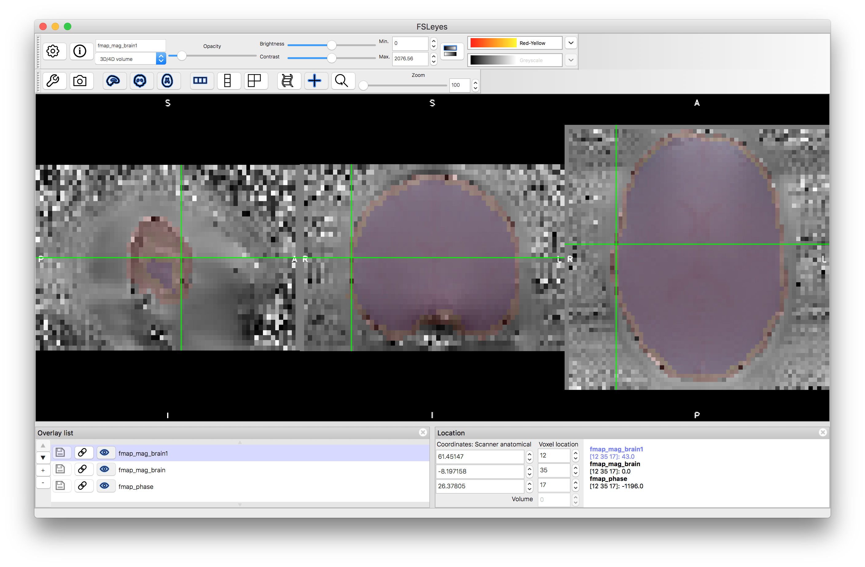
The second step here is necessary to remove noisy edges from phase image but is not necessary in all datasets. Inspect the results of these two brain extraction steps: fmap_mag_brain1.nii.gz and fmap_mag_brain.nii.gz to see the difference, and also load the fmap_phase.nii.gz image to see the noisy values at the edge (e.g. give the two brain extractions different colours, make them quite transparent, and put them on top of the phase image - so that you can see if the brain extractions cover the noisy voxels at the edge or not - see image below).
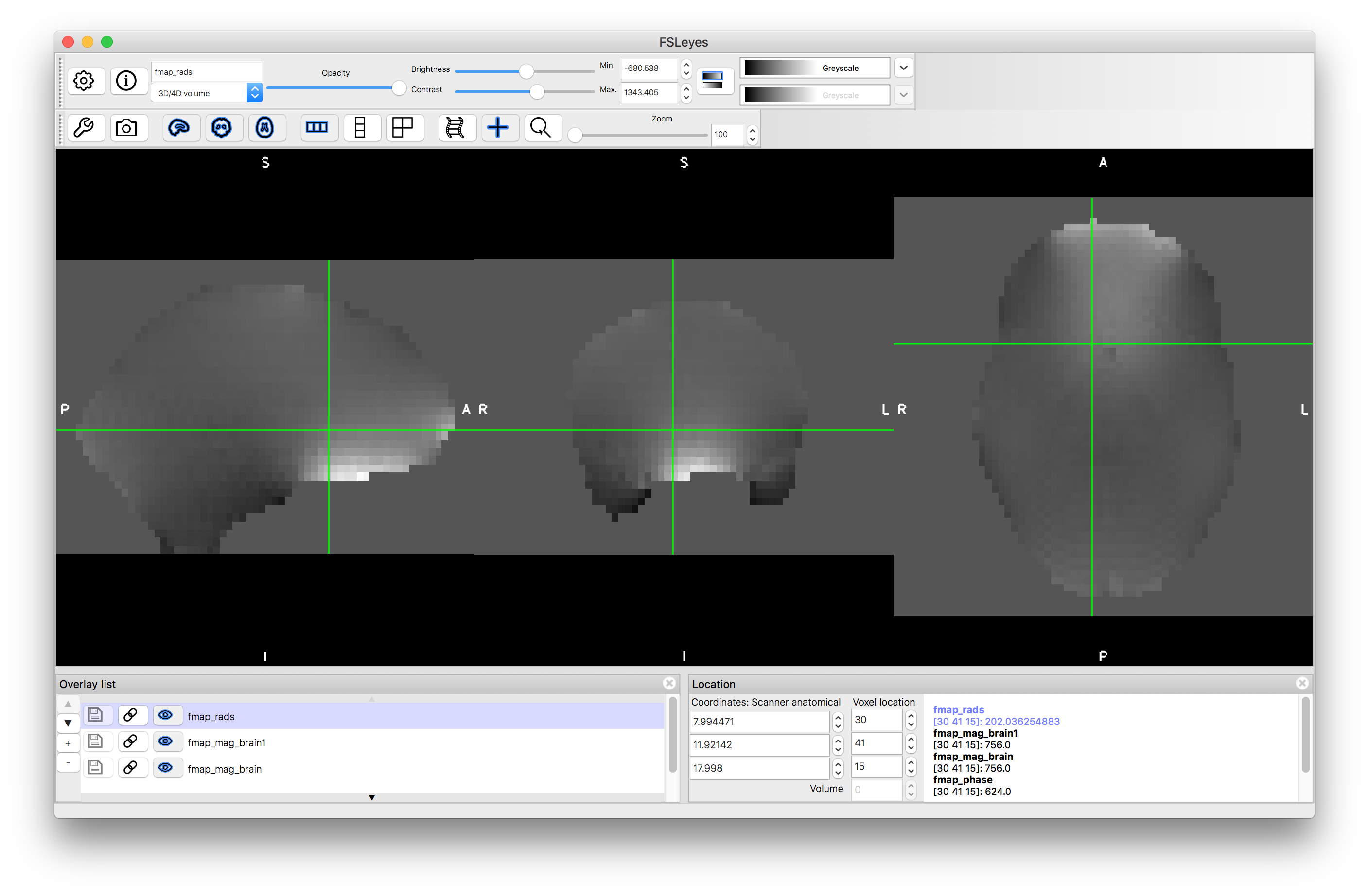
The third command above performs some masking and scaling operations to the phase image, to covert it into the required units of radians per second (denoted by rads in the filename). For this it needs to know one key parameter value, which is the difference in echo times used within the fieldmap acquisition. In this case it was 2.46 milliseconds, but this may vary on different scanners and at different sites, so ask your scanner operator to provide you with this value when you do your own fieldmap scans (if you use the gradient-echo style - see another example box for details on the blip-up-blip-down alternative). View the output fmap_rads - it should look very similar to the phase image, just masked and with the intensities scaled differently.
BBR registration
Now that the fieldmap is in the required format we can apply the BBR registration of the EPI to the structural, using the fieldmap information to correct for geometric distortion. In order to do this we need to have a segmentation of the structural image, in order to find the white matter edges. Here this segmentation is provided for you in the image T1_wmseg.nii.gz but this can easily be calculated from the T1-weighted image in FSL using the FAST tool.
To run the BBR registration also requires a parameter from the EPI sequence - the effective echo spacing (also known as "dwell time"). This is the amount of time it takes to acquire lines in k-space (though you do not need to understand what this means). Your scanner operator will be able to provide you will this value. It is typically around 0.3 to 1.0 milliseconds for most modern sequences. If you are using in-plane acceleration (e.g. GRAPPA or SENSE) then the raw echo spacing needs to be divided by the acceleration factor to get the "effective echo spacing". For this particular sequence it is 0.5 milliseconds. Remember that this is a parameter of the EPI sequence (i.e. the fMRI or dMRI acquisition) and not the fieldmap sequence.
In FSL there is a specific script used for applying BBR registration (with or without fieldmaps) to EPI images - epi_reg. This also needs to know the phase encoding direction in the EPI image, in terms of voxel coordinates. In this case it is the y-direction and the distortion is in the negative y-direction, though knowing whether it is positive or negative is extremely tricky to figure out a-priori and the recommended way to determine this in practice is just to try both positive and negative and see which one gives the better distortion correction. The specific command for this example is:
epi_reg --echospacing=0.0005 --wmseg=T1_wmseg.nii.gz --fmap=fmap_rads.nii.gz \
 --fmapmag=fmap_mag.nii.gz --fmapmagbrain=fmap_mag_brain.nii.gz --pedir=-y \
 --epi=func.nii.gz --t1=T1.nii.gz --t1brain=T1_brain.nii.gz --out=func2struct
The backslashes at the end of end line are just a convenient way to continue the same command over several lines (so keep them in if you are copying and pasting, but if you are typing it out in one line then leave them out). Also, note that the output name does not have .nii.gz after it in this case, as it is used as the prefix for a host of output names.
After you have run the above command (and it will take a while to run) list the contents of the current directory (use ls in the terminal, or view it in a graphical file browser) to see the outputs that are created (they start with the specified prefix func2struct). The main outputs are a version of the functional image that is aligned and resampled into the structural space (func2struct.nii.gz) as well as spatial transformations (func2struct.mat - from undistorted functional space to structural space; and func2struct_warp.nii.gz - from distorted functional space to structural space) - the other outputs you can ignore.
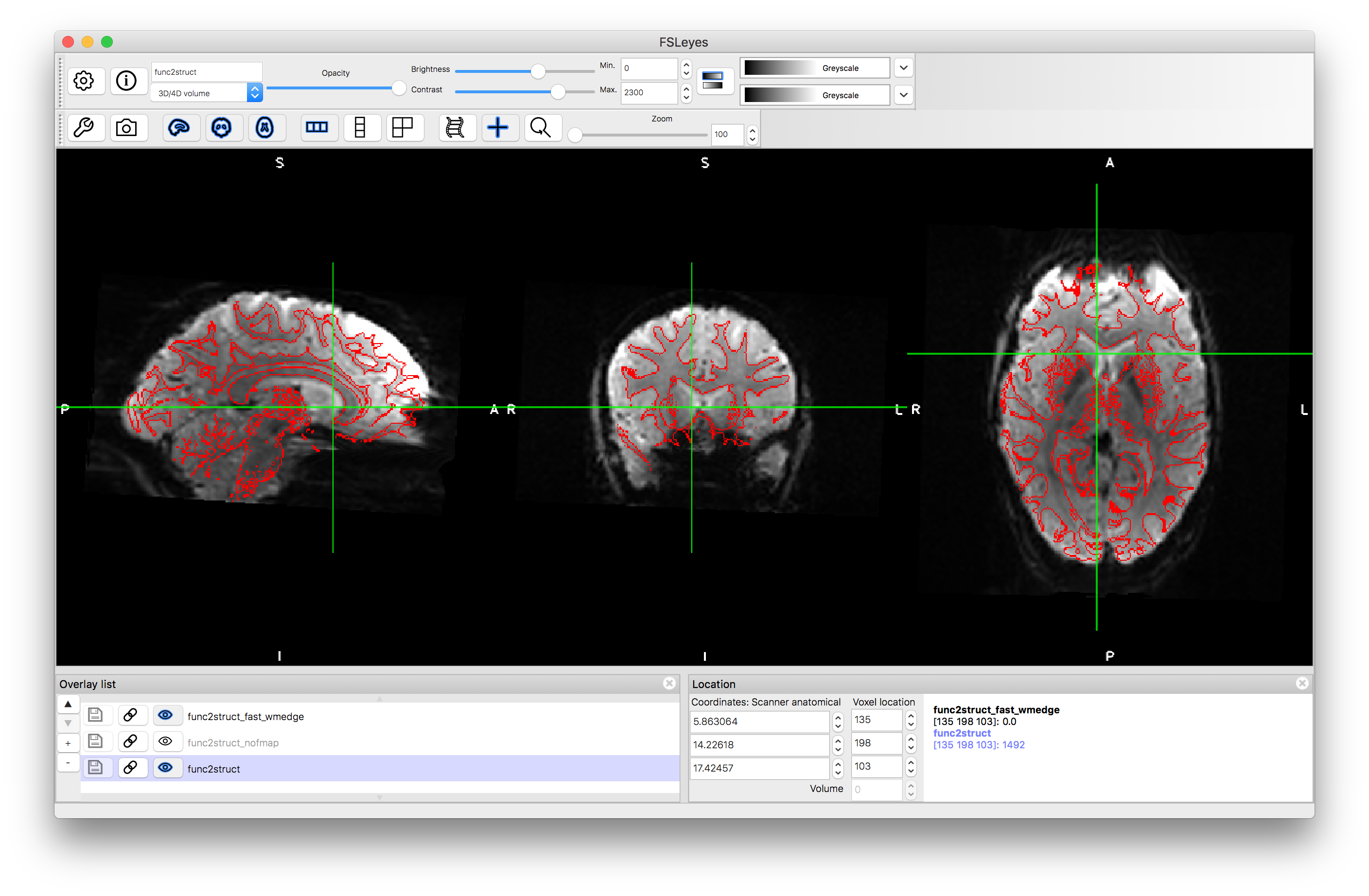
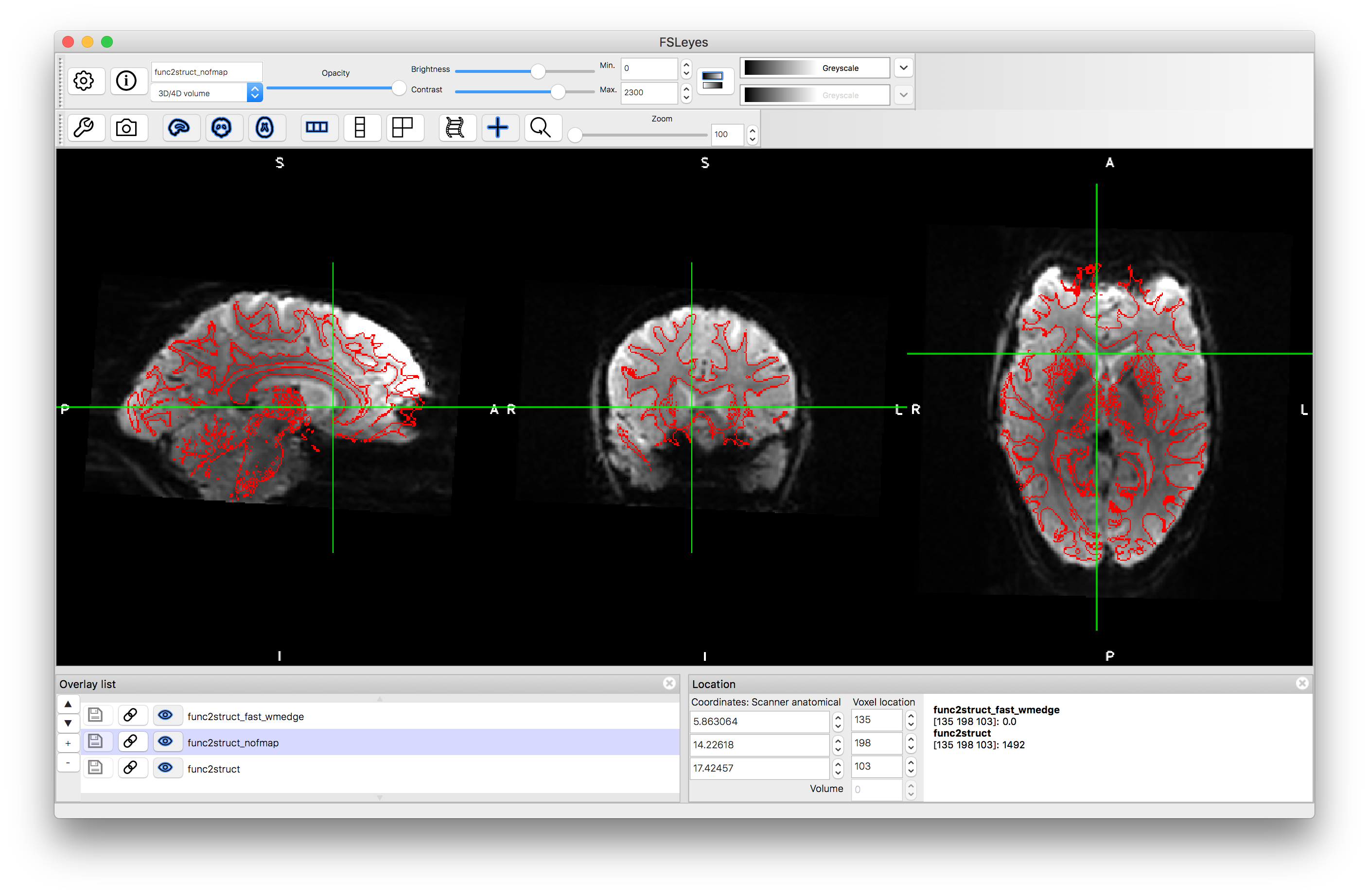
Load the output func2struct.nii.gz and compare this to the T1-weighted structural image T1.nii.gz. You can add the red edges (boundaries of the white matter) by loading func2struct_fast_wmedge.nii.gz. This corresponds to the distortion corrected results shown in Figure 6.6. It is useful to compare this result to a BBR registration result without using fieldmaps for distortion correction - this is provided as pre_baked/func2struct_nofmap.nii.gz that you can load (or you can create it by running epi_reg without fieldmaps ). If you keep the red edges on top and toggle between the registration results with and without distortion correction (using the "eye" icon to turn the images on and off) then you can clearly see what the distortion correction does. This helps to improve the alignment substantially in areas such as the anterior ventricles and inferior regions, although it has minimal impact in other areas. Where there is substantial signal loss it is difficult to assess the accuracy of the registration, since the edge of the visible tissue corresponds to an arbitrary signal loss boundary and not a true anatomical boundary.
With distortion correction:
Without distortion correction:
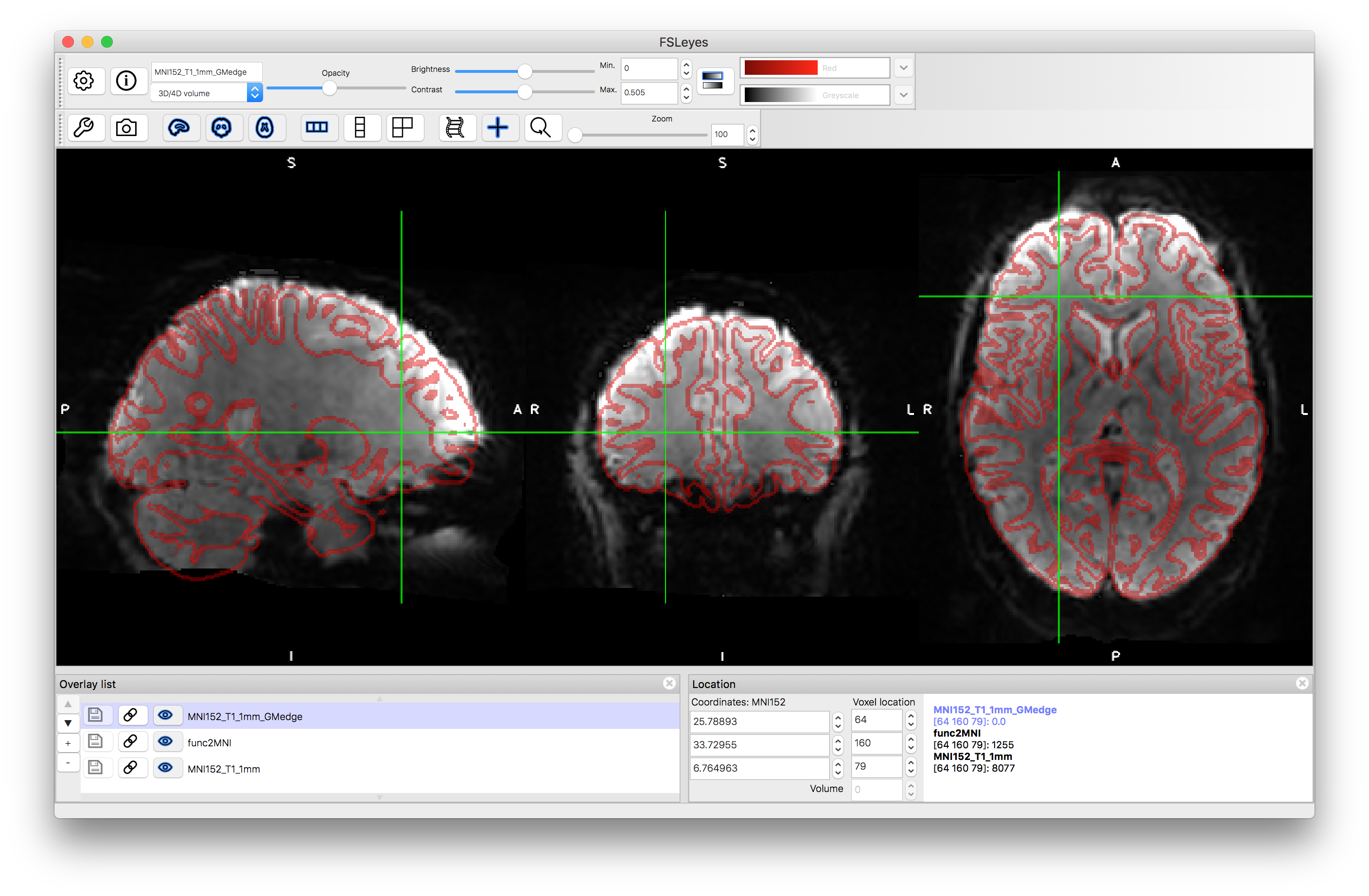
Combining transformations
To create a version of the functional image in the standard space we need to combine the functional to structural transformation with the structural to standard transformation. This can be done in FSL with the following commands:
convertwarp -r $FSLDIR/data/standard/MNI152_T1_1mm.nii.gz --warp1=func2struct_warp.nii.gz --warp2=T1toMNI_warp.nii.gz -o func2MNI_warp.nii.gz
applywarp -i func.nii.gz -r $FSLDIR/data/standard/MNI152_T1_1mm.nii.gz -w func2MNI_warp.nii.gz --interp=spline -o func2MNI.nii.gz
The first command combines the two warps together and the second applies the combined warp to resample the functional image into the standard space. Inspect the output by loading the result func2MNI.nii.gz along with the standard MNI template MNI152_T1_1mm.nii.gz and the grey matter edges MNI152_T1_1mm_GMedge.nii.gz. You should find the major anatomical features are well aligned although some inaccuracies in the smaller folds and in areas where there was signal loss, which will still be present.
From these examples you should be able to replicate the three case studies from section 5.4, and all the panels in Figure 5.11, with versions of the functional image in all spaces (functional, structural and standard), and versions of the structural image in structural and standard space. The above commands are general and can be applied (with possible minor modifications) to images of other subjects as well as to other EPI images (e.g. dMRI). Although the commands above are specific to FSL, these principles will apply generally in other software packages too.