Example Box: Viewing Diffusion Images
Introduction
The aim of this example is to become familiar with what diffusion images look like and how relevant information is encoded in them.
This example is based on tools available in FSL, and the file names and instructions are specific to FSL. However, similar analyses can be performed using other neuroimaging software packages.
Please download the dataset for this example here:
Data download
The dataset you downloaded contains the following files:
- Diffusion images:
data.nii.gz - Two text files:
bvalsandbvecs - A separate (partial) set of diffusion images:
b1500.nii.gz
data.nii.gz).
Viewing the Data
To start with load the diffusion images into a viewer (e.g. fsleyes) and inspect the image. The resolution is not as high as a structural image (the voxel size is 2x2x2 mm in this case) and so the anatomy is not quite as clearly defined. The data here contains 64 separate images, and you can view each one by either changing the "Volume" number (in the box at the bottom, underneath the voxel coordinates) or by using movie mode (use movie icon) - see red circles on image below.
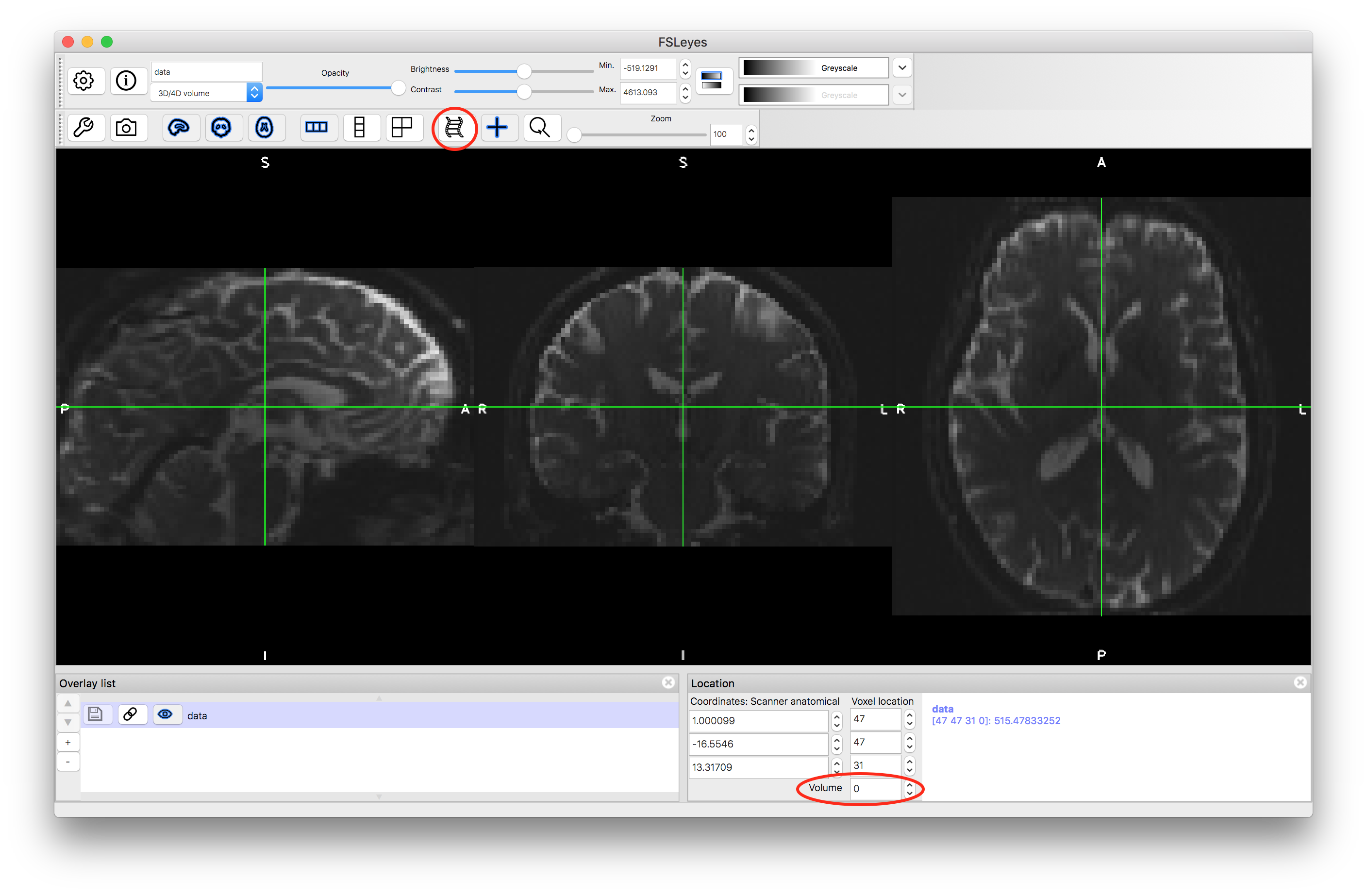
When stepping between volumes the most obvious change is the large change in intensity between the non-diffusion-weighted images (such as volume number 0) and the diffusion-weighted images (volumes 1, 2, etc.). To see the details in the diffusion-weighted images it is usually necessary to reset the brightness and contrast controls. Set the volume to number 5 and increase the brightness and contrast (use the sliders) until you can see the intensities more clearly (such as in the image below).
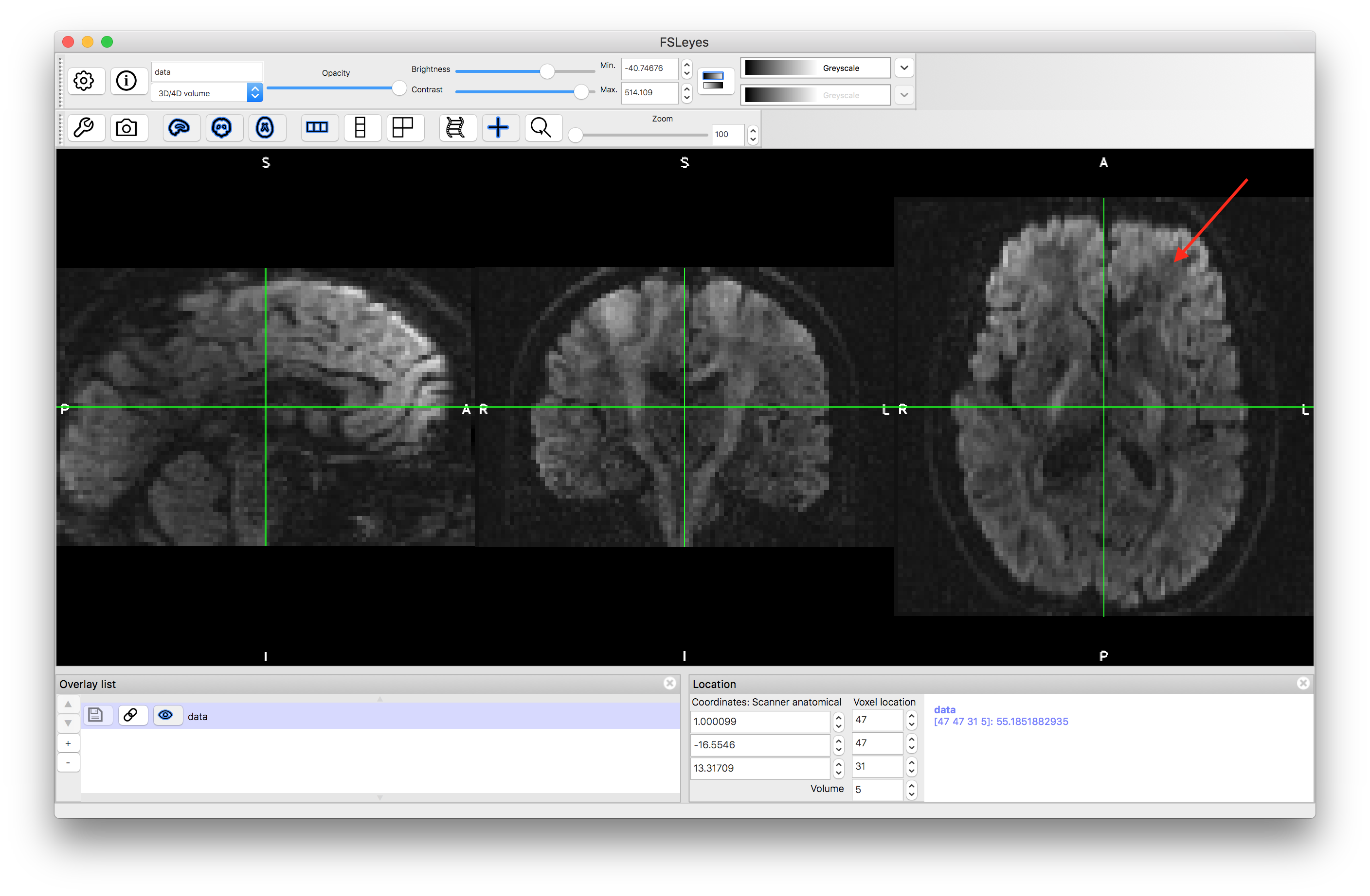
If you compare volume 5 to volumes 4 and 6 you will be able to see that the portion of the axial slice in the top right part (the Left Anterior portion - see arrow) near the ventricles is darker in volume 5, following the diagonal fibre pathways in this area of the anatomy. This reduction in intensity is how the information about the direction of the diffusion is encoded in the images. It indicates that for this particular volume (number 5) the voxels where the intensity is reduced correspond to locations where the diffusion is along the direction associated with diffusion encoding direction that was applied for this volume. The information about the diffusion directions is pre-specified in the imaging sequence that is used to acquire the data. This information can also be found in the bvals and bvecs files.
B-values and Encoding Directions
The first six values in the bvals file are:
0 1500 1500 1505 1495 1500
which indicates that the first volume (volume number 0) has no diffusion weighting (as the b-value is zero), whilst the others have diffusion weighting (with a b-value of roughly 1500). This is also obvious from looking at the images, since the first image (volume number 0) is much brighter than the others (as the diffusion weighting reduces the overall intensities).
The first six values in the bvecs file (which has three lines) are:
0  0.99998354911804 0.57847899198532 0.20246583223342 -0.34904509782791  0.58626478910446
0 -0.00333316996693 0.67102438211441 0.41539564728736  0.16653540730476  0.79655337333679
0  0.00466644018888 0.46377617120742 0.8868224620819  -0.92218953371048 -0.14763586223125
which indicates that for volume 5 (the sixth values), the direction of the diffusion encoding is represented by the vector (0.586, 0.797, -0.148). This vector has its largest values in the x and y directions, meaning that it is pointing at roughly 45 degrees within the axial plane, as we saw in the top right part of the axial slice before.
Tissue Type Dependence
If you run the movie mode (or just change the volume numbers by hand) you will see that voxels in the ventricles, that contain CSF, are very bright in the non-diffusion-weighted images but dark in all the diffusion-weighted images. This is due to the fact that in CSF water is free to move in any direction and so the intensity reduces regardless of what the encoding direction is. This is also true in gray matter, but to a lesser extent (as water moves equally in all directions on average within gray matter, but not as freely as in CSF).
In white matter the reduction in intensity is highly dependent on the direction of the diffusion encoding, according to whether the white matter tract (axonal fibre bundles) are in the same direction as the diffusion encoding or not. When the directions are the same (as for the fibre bundles in the top right portion of volume 5) then the intensity is substantially reduced, by comparison with the intensity in case when the directions are different. In this way the fibre bundle direction at a particular voxel can be calculated, as the volume with the lowest intensity will be the one where the encoding direction is closest to the actual fibre bundle direction.
Artifacts
The dataset above contains a minimal amount of the two main artifacts seen in diffusion imaging: eddy current distortion and susceptibility-induced distortion (due to B0 inhomogeneities). Now load the second dataset b1500.nii.gz into the viewer (or a separate viewer). This is a partial dataset (containing only some of the diffusion-weighted images and none of the non-diffusion-weighted images) but shows the artifacts more clearly.

In the image above you can see the circled area which illustrates the geometric distortion (or susceptibility-induced distortions) associated with B0 inhomogeneities. Note that there is a bright rim here where the signals that have been pushed down from above (in the A to P direction) pile on top of each other.
Eddy-current distortions are difficult to identify in individual images but if you turn on movie mode then you can see that the whole brain tends to move about in the image frame. This can be easier to see if you put the crosshairs on a point on at the edge of the brain, as you can see the edge movement with respect to this fixed point. Such shifts can also be due to movement, although eddy currents can also stretch the image.
These examples, together with the explanation and examples in the Primer text should help you to understand the relationship between the intensities and the directional information about axonal fibre bundles.