Example Box: Deep Gray Matter Structure Segmentation
Introduction
The aim of this example is to perform a segmentation of several deep gray matter structures and understand the outputs and options available.
This example is based on tools available in FSL, and the file names and instructions are specific to FSL. However, similar analyses can be performed using other neuroimaging software packages.
Please download the dataset for this example here:
Data download
The dataset you downloaded contains the following files:
- Original structural data:
T1.nii.gz - A directory of pre-baked results:
pre_baked_res
Viewing the Data
To start with load the original structural image T1.nii.gz into a viewer (e.g. fsleyes) and inspect this. There is some noticeable bias field in the superior portion of the image, but nothing that will be problematic for deep gray matter segmentation.
Running the Segmentation
You can easily perform a segmentation using the FSL tool FIRST. To do this you can run it from a terminal - just use cd to change directory to the location where this data is and then run the command:
run_first_all -i T1.nii.gz -o T1seg
Alternatively, you can just look at results that we have already generated in pre_baked_res.
Viewing the Results
Several deep gray matter structures are segmented by FIRST: Brainstem, Nucleus Accumbens, Amygdala, Caudate, Hippocampus, Pallidum, Putamen, Thalamus. These are separately segmented in the left and right hemispheres except for the brainstem.
The results are stored in several different formats, but the two that are the most useful are: T1seg_all_fast_firstseg.nii.gz and T1seg_all_fast_origsegs.nii.gz. In the former there is a single 3D image where all structures are labelled (each voxel contains one number that, if greater than zero, indicates which structure it is part of: e.g., 10 for left Thalamus, 11 for left Caudate, etc. In the latter, each structure is represented by a separate 3D image (stored as multiple volumes within a 4D image) and each volume has separate labels for the interior of the structure and voxels on the border. We will look at these in more detail now.
Boundary Corrected Results
Load the image T1seg_all_fast_firstseg.nii.gz in the same viewer as the T1.nii.gz image. This should show all the structures together with different colours (if not, set the colormap to "MGH Sub-cortical") and you can click around to see the quality of the segmentation - you may like to reduce the opacity of the segmentation to get a better view of the underlying anatomy. In many places within the image there is insufficient intensity contrast to determine the boundary location (e.g., the lateral boundary of the thalamus) and in these cases the segmentation will resort to the information it learnt about the typical shape of that structure in the general population. Another point to note is that the brainstem involves some arbitrary cutoffs (these were part of the protocol used to define the brainstem in the manual segmentations that this method was trained on).
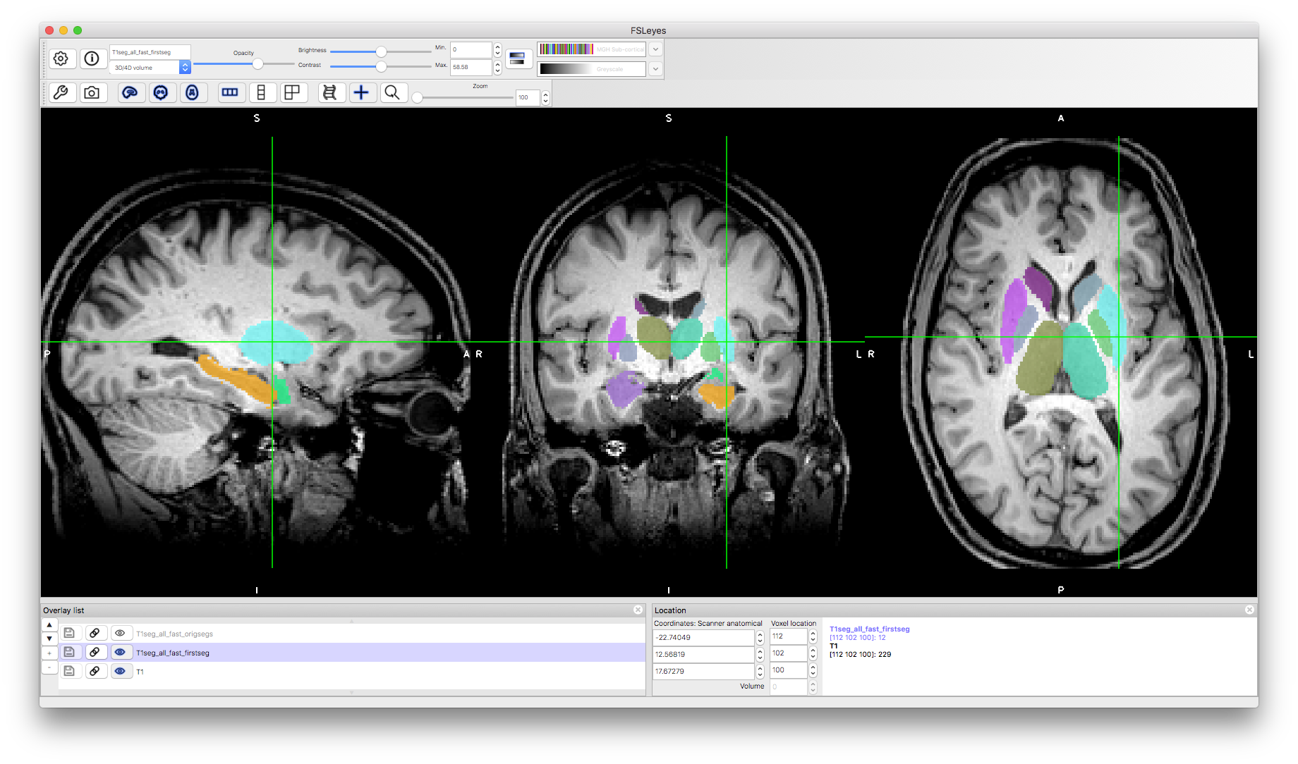
This form of segmentation is useful for defining ROIs and other masks for use in analysis pipelines. It is also possible to perform analysis of the geometry of the structural segmentations, but in that case other geometry information is used (in the bvars and vtk files).
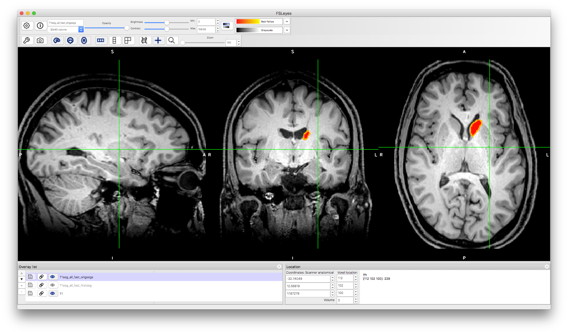
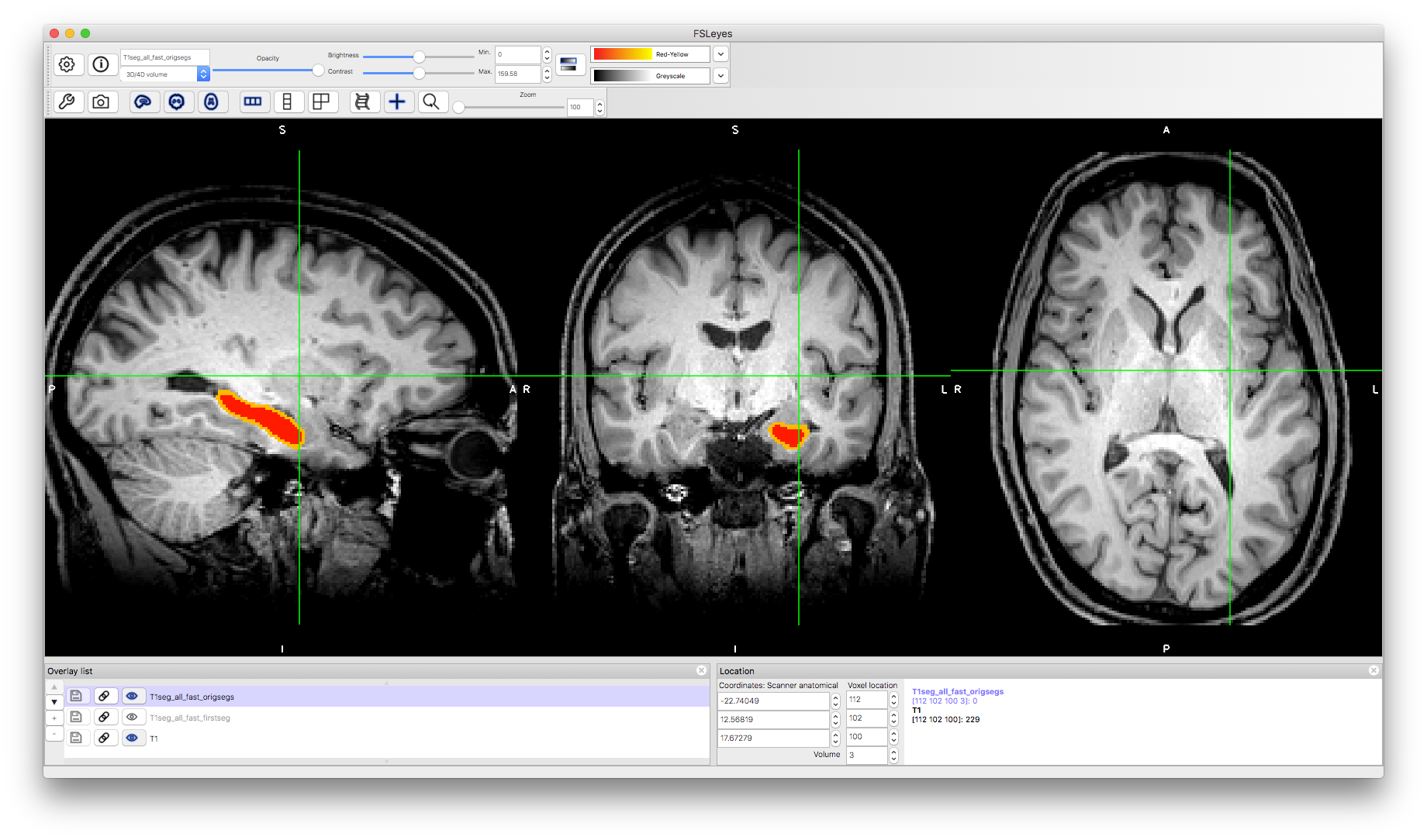
Individual Structure Segmentations
The other form of segmentation result shows the separation of voxels classified as in the interior of the structure versus those where the mesh that represents the boundary passes through the boundary voxels. To see this, load the image T1seg_all_fast_origsegs.nii.gz on top of the other images. Change the "Volume" number to see different structures. For instance, volume number 2 is the left caudate and volume number 3 is the left hippocampus, as shown below. In each case (if you set the colourmap to Red-Yellow) then the interior is shown in red and the border in orange/yellow.
This image allows you to inspect whether the boundary is correctly located as well as to evaluate the performance of the boundary correction procedure. The previous output was the result of performing this boundary correction procedure, where each boundary voxel is reclassified as either belonging with the interior voxels of that structure, or as part of a neighbouring structure. There are alternative options for boundary correction (the command above uses the default option) and in some circumstances it can be helpful to use an alternative (e.g., for applications where it is more important to be inclusive rather than exclusive). If the non-boundary voxels are incorrectly classified then none of the boundary correction options can fix this. Hence this image is useful when evaluating and optimising performance.
Caudate
Hippocampus
Multimodal Segmentation
Another tool in FSL for segmenting deep gray matter structures is MIST. This relies on a training set consisting of a number of subjects, each with a set of images of multiple modalities (e.g., T1-weighted, T2-weighted and diffusion), as well as one example segmentation of the structure of interest. From this the method learns how to identify useful intensity features (from one or more of the imaging modalities) at each point on the structure's boundary. See the FSL wiki page for more details about this method. If you have a dataset with multiple modalities then you can also try this method on your data.
This example should give you some experience of perform deep gray matter segmentation, some of the options available, and the types of output to expect. More details on any of the methods in FSL can be found on the FSL wiki.