Example Box: Correcting for Distortions and Artifacts in Diffusion Images
Introduction
The aim of this example is to become familiar with what kind of artifacts are present in diffusion data and the ability of the pre-processing pipeline to correct for these given appropriate data.
This example is based on tools available in FSL, and the file names and instructions are specific to FSL. However, similar analyses can be performed using other neuroimaging software packages.
Please download the dataset for this example here:
Data download
The dataset you downloaded contains the following files:
- Non-diffusion-weighted images with two phase encodings:
AP_PA_b0.nii.gz - Distortion correction non-diffusion-weighted images:
topup_AP_PA_b0_iout.nii.gz - Original diffusion-weighted data:
b1500.nii.gz - Eddy-current and distortion corrected data:
eddy_unwarped_images_b1500.nii.gz
Viewing the Data
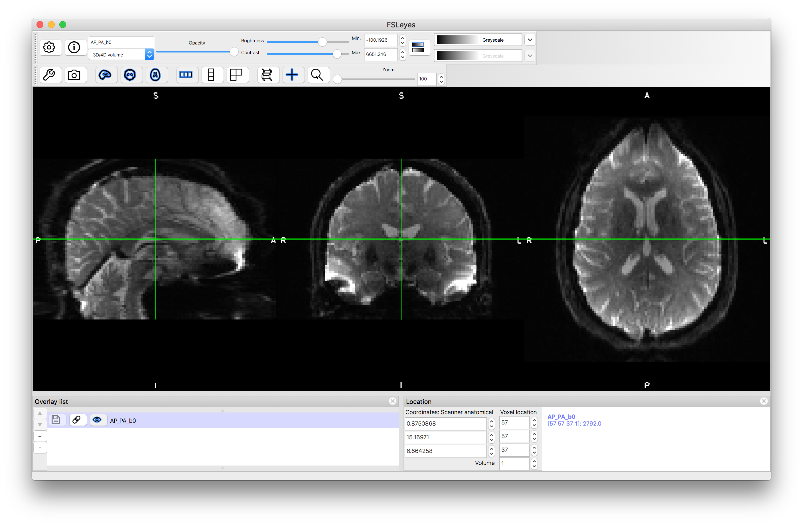
To start with load the original non-diffusion-weighted (b=0) images AP_PA_b0.nii.gz into a viewer (e.g. fsleyes) and inspect these - you may need to adjust the brightness and contrast for this and other images in this example. This is actually a 4D image where two 3D volumes have been put together in the same file for convenience. You can see each individual image by changing the "Volume" number (it can be either 0 or 1 in this case). The difference between the two images should be obvious in the anterior portion of the brain where there is substantial geometric distortion due to the presence of B0 inhomogeneities induced by the air-filled sinuses.

Distortion Correction
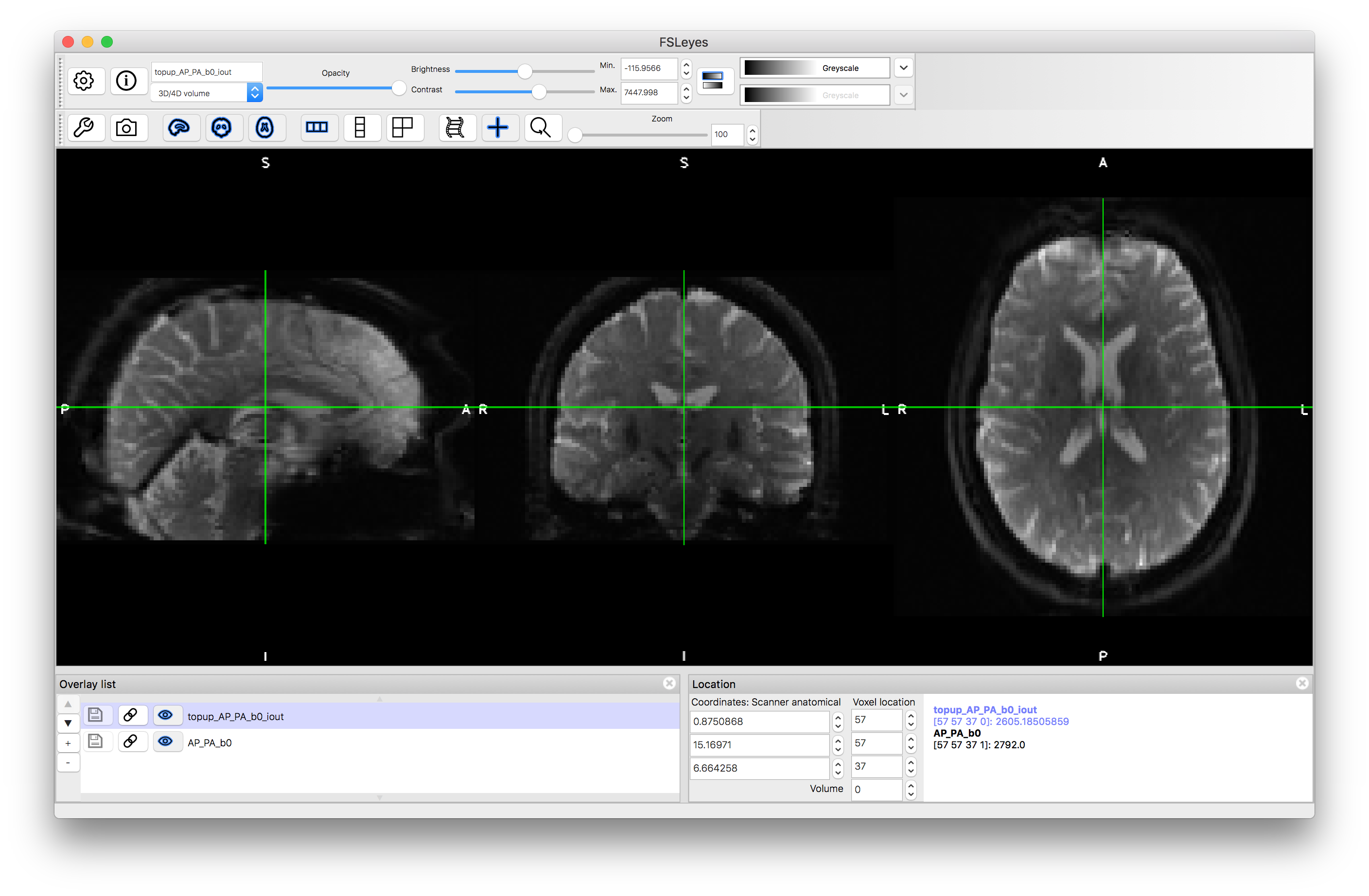
These distortions are significant artifacts that seriously affect the quality of diffusion quantification, the tractography and the alignment that can be done using this data. However, the FSL tool topup can take this data (phase-encode b=0 reversed pair) and calculate a corrected image from them (or, ideally, even more repeats of these b=0 image pairs). Load topup_AP_PA_b0_iout.nii.gz which shows the result of running topup on this data. This method of calculating and correcting the distortions due to B0 inhomogeneities (also known as susceptibility induced distortions) is covered in more detail in chapter 6 of the Primer. For now just note how well the method corrects for the geometric distortion.
Eddy-Current Correction
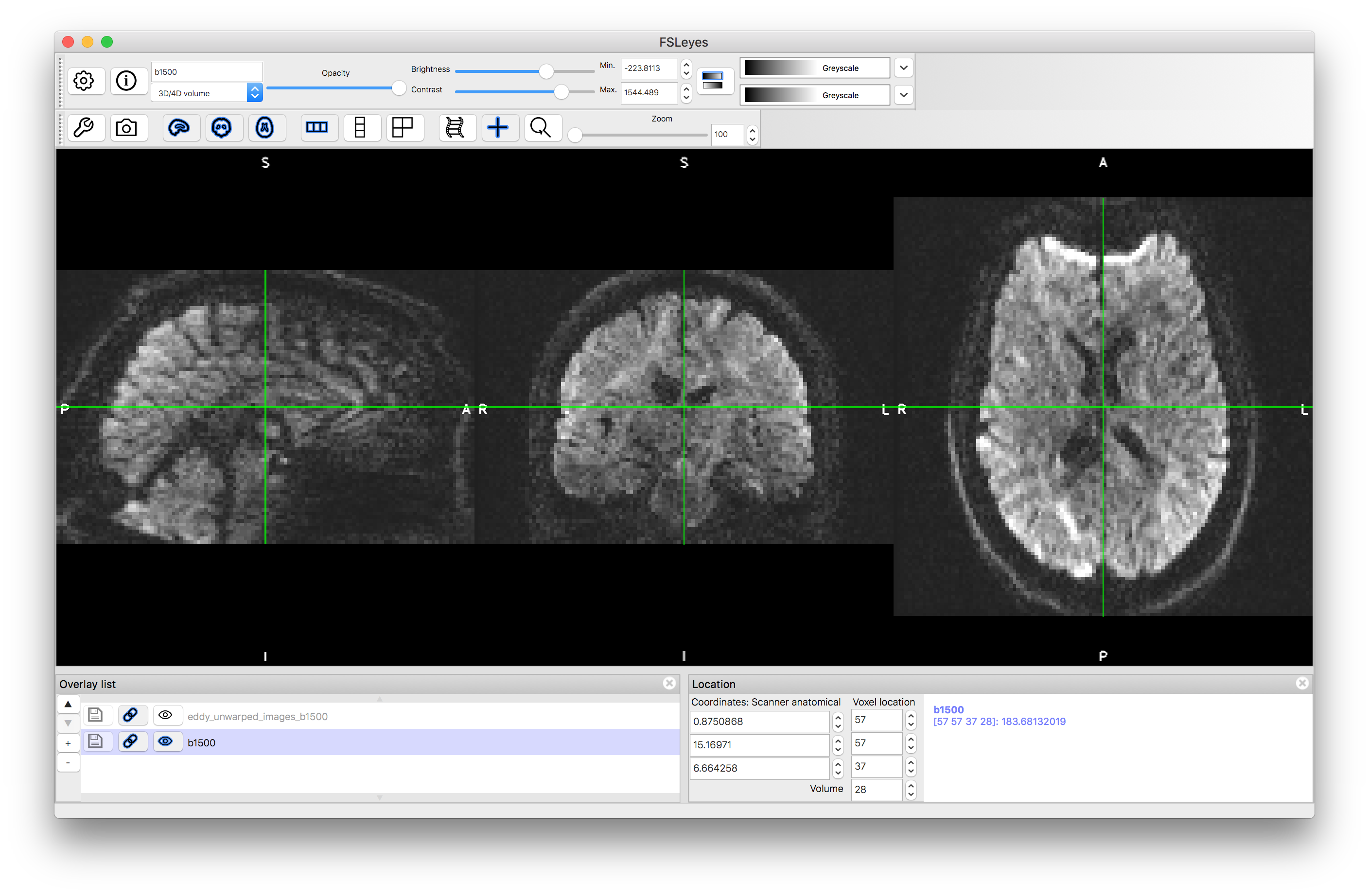
Now open the image b1500.nii.gz in a separate viewing window. This data contains only the diffusion-weighted images from a dMRI acquisition (i.e., the non-diffusion-weighted images have been stripped out). Once you have adjusted the brightness and contrast turn the movie mode on and watch how each 3D image differs from the others - both in terms of diffusion contrast, where the intensity undergoes great changes in the white matter depending on the encoding direction, but also in terms of movement of the whole image. This movement is mixture of actual subject motion and eddy-current distortions (which appear as global shifts and scalings rather than local distortions).
Load the image eddy_unwarped_images_b1500.nii.gz and view this in movie mode. You should see that although the changes in intensity due to the diffusion encoding is still present, the images display much less motion. This is because this image is the output of the tool eddy, which corrects for eddy-current-induced distortions as well as for subject motion and also for distortions due to B0 inhomogeneities. The latter is corrected for by utilising information supplied by topup and so requires the same input data (phase-encode reversed b=0 image pairs). Corrections for eddy-current-induced distortions and subject motion are estimated by eddy directly from the diffusion-weighted data together with information about the b-values and diffusion encoding directions (also known as b-vectors). An important point to note here is that the quality of the eddy-current correction is better when the directions are distributed over a full sphere (as opposed to a half sphere) as explained in the Primer.
If you link the two images (using the "chain" icon, to the left of the "eye" icon, that is to the left of the image name in the Overlay list) then you can also turn the top image on and off in order to flick between the correct and uncorrected versions. This can more obviously show you how much distortion and motion has been corrected. Try this for different volumes, as the eddy-current distortions are different for each volume, since they depend on the diffusion encoding gradients (which are made to vary from volume to volume).
Before Correction
After Correction

This example demonstrates the magnitude of the artifacts in diffusion data, why it is important to correct for these and how well the correction methods can work. It is important that these methods are provided with the correct data (e.g., phase-encode reversed b=0 pairs) in order to be able to perform the correction. Otherwise the artifacts would have a significant negative impact on the analysis. More details about the topup and eddy method and how they are applied to this dataset can be found at FSL course website in the "FDT & TBSS Practical".