Example Box: Tractography
Introduction
The aim of this example is to run probabilistic tractography on some real data and understand how this, together with different seeds and masks, can be used to delineate anatomical tracts.
This example is based on tools available in FSL, and the file names and instructions are specific to FSL. However, similar analyses can be performed using other neuroimaging software packages.
Please download the dataset for this example here:
Data download
The dataset you downloaded contains the following files:
- A directory containing a lot of outputs from pre-processing:
subj1_model2_3fibres.bedpostX - A directory containing some already calculated results:
pre_baked
Viewing the Data
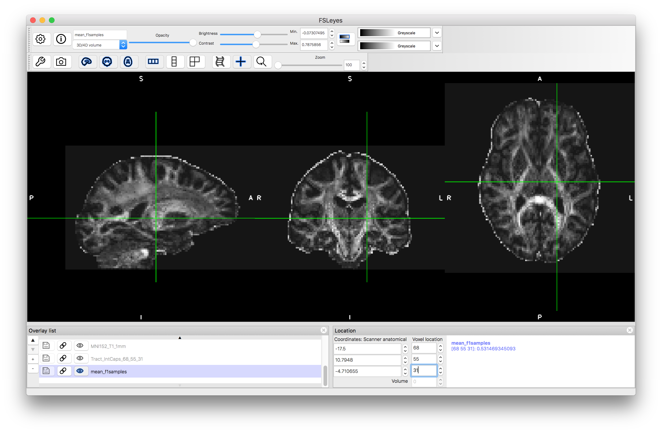
To start with load the image mean_f1samples.nii.gz into a viewer (e.g. fsleyes). This is an image of an anisotropy parameter in the ball-and-sticks diffusion model and provides information that is similar to the FA map from the diffusion tensor model. We load this first in order to give us a visual reference for the brain.
Tractography from a Single Seed
Let us start by running tractography from a single seed location (you can compare with the results in the pre_baked directory)). Pick a point in a strong tract, such as the internal capsule: e.g., we chosen voxel coordinate (68, 55, 31) but feel free to choose any point you like.
We will now use the FSL tool probtrackx (that is part
of FDT - the FMRIB Diffusion Toolbox) to perform tractography. This
is done using the following steps:
- Start the main FSL GUI by typing
fsl &in a terminal. - Select the FDT tool
- In the new FDT GUI, use the top pull down menu to select the "PROBTRACKX" option
- Use the file browser to select the directory containing the
subj1_model2_3fibres.bedpostXdirectory - Enter the chosen voxel coordinate in the "Seed Space", making sure that the pull down menu is set in the "Single voxel" mode
- Put in an output name (this we be a directory that contains output files)
- Press "Go"
- Wait for a popup box telling you it is finished, or monitor the progress in the terminal window.
Load the results of this into fsleyes, by finding the appropriate image file in your output directory - it will have a name something like TractIC_68_55_31.nii.gz (where the "TractIC" part will be the name of your output directory). Give this result a colour and set the "Min" display range to 50.
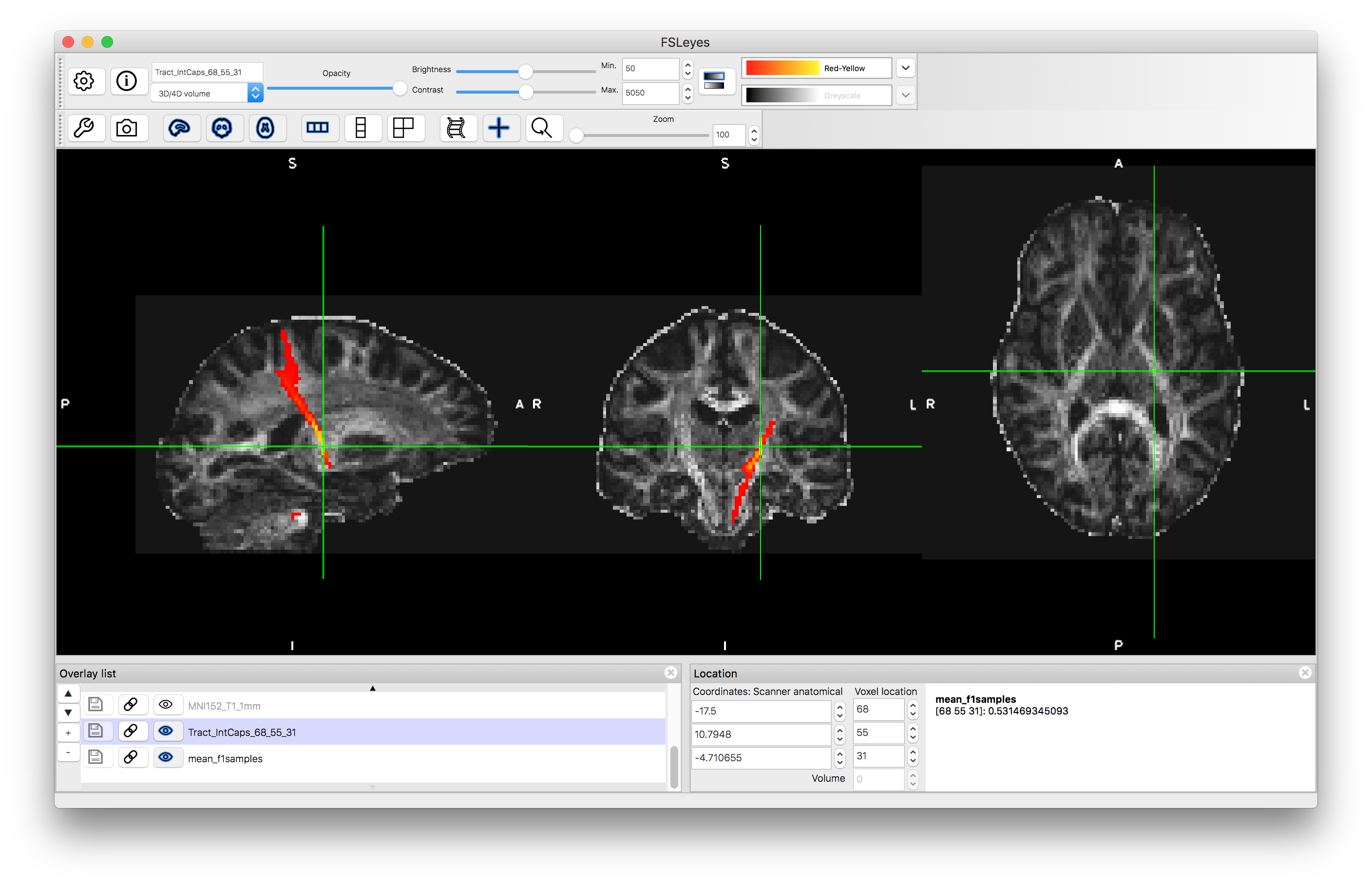
If you change the "Min" value to a much lower value (e.g., 5) then you will see an increase in the number of voxels that are included in the tract. This is because the result is a probabilistic tractography result and the "Min" value is acting to remove voxels with low probability of being in the tract. The actual values stored are a count of the number of streamlines running through a voxel (the number of times a randomly sampled tract passes through the voxel). By default 5000 samples are generated and so the values can go up to this, such that 50 represents a 1% probability and 5 represents a 0.1% probability. Hence the voxels that are not shown when "Min" is set to 50 are those voxels that have a probability (of being part of the tract) of less than 1%. Unlike statistical tests, there is no defined standard for thresholding these probabilities, as it will depend on what the output is being used for.
Feel free to try seeding from other locations and see what the results look like. If you seed from something that is within a clear, major tract then the results can often be very messy.
Tractography using Masks
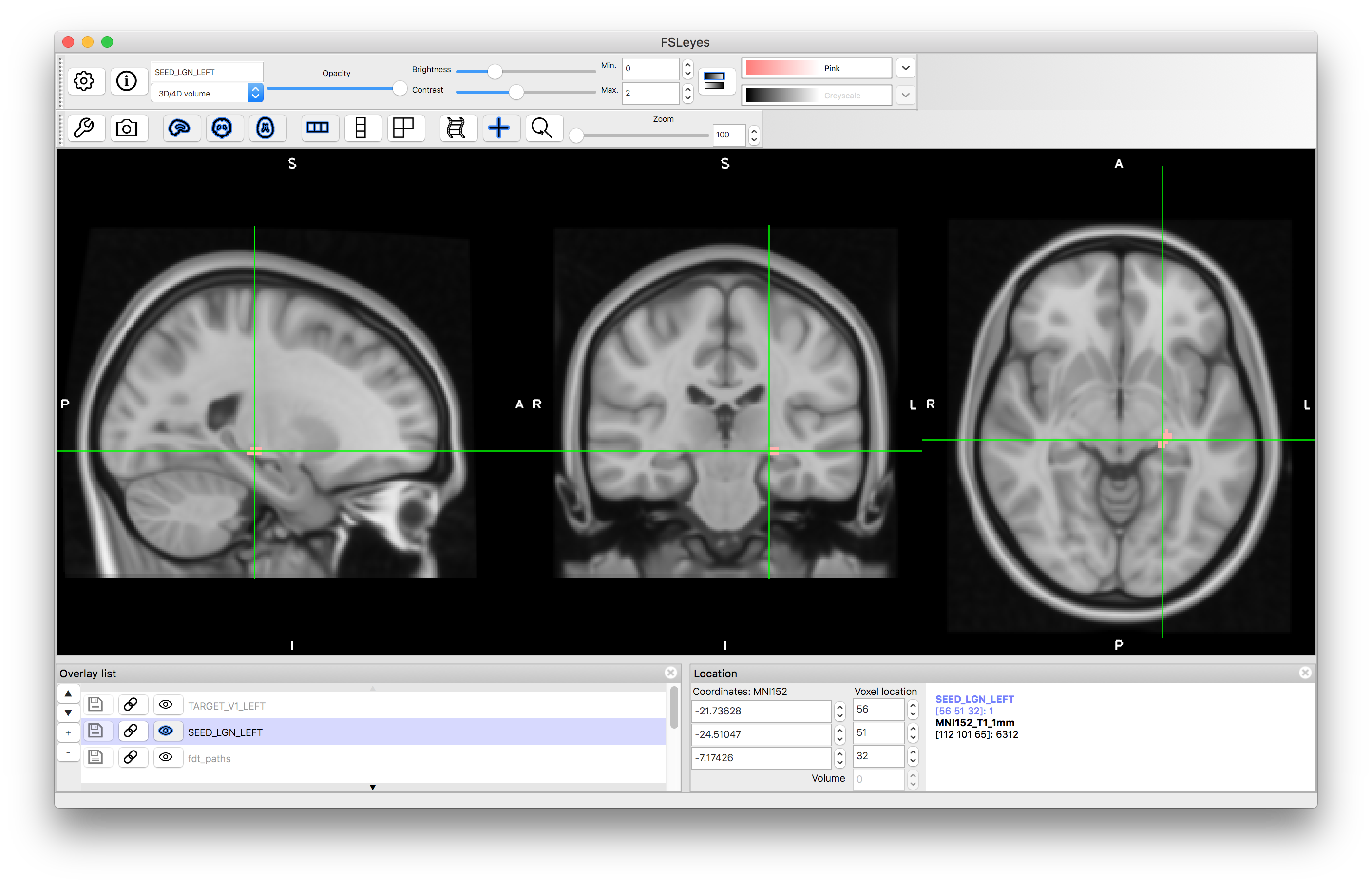
Now we will run tractography to delineate the optic radiation by seeing from the lateral geniculate nucleus of the thalamus (LGN) and looking for connections to primary visual cortex (V1). A mask that defines the LGN is contained in the directory and is called SEED_LGN_LEFT. This mask is in standard space, and so we will run this tractography in standard space.
Open a new viewer window and load the standard image MNI152_T1_1mm (use the "Add standard" option from the File menu in fsleyes). Once this is loaded, add the SEED_LGN_LEFT image and view this.
We will use this mask to run tractography by using the following steps:
- Start the main FSL GUI by typing
fsl &in a terminal. - Select the FDT tool
- In the new FDT GUI, use the top pull down menu to select the "PROBTRACKX" option
- Use the file browser to select the directory containing the
subj1_model2_3fibres.bedpostXdirectory - Using the pull-down menu, change "Single voxel" to "Single mask" under "Seed Space"
- Use the file browser to select the
SEED_LGN_LEFTimage as the "Seed Image" - Select the "Seed space is not diffusion" button (as our seed is in standard space)
- Select the "nonlinear" checkbox
- Use the file browser to enter
standard2diff_warp.nii.gzin the "Select Seed to diff transform" box (this file is in thexfmssubdirectory) - Use the file browser to enter
diff2standard_warp.nii.gzin the "Select diff to Seed transform" box (this file is in thexfmssubdirectory) - Put in an output name (this we be a directory that contains output files)
- Press "Go"
- Wait for a popup box telling you it is finished, or monitor the progress in the terminal window.
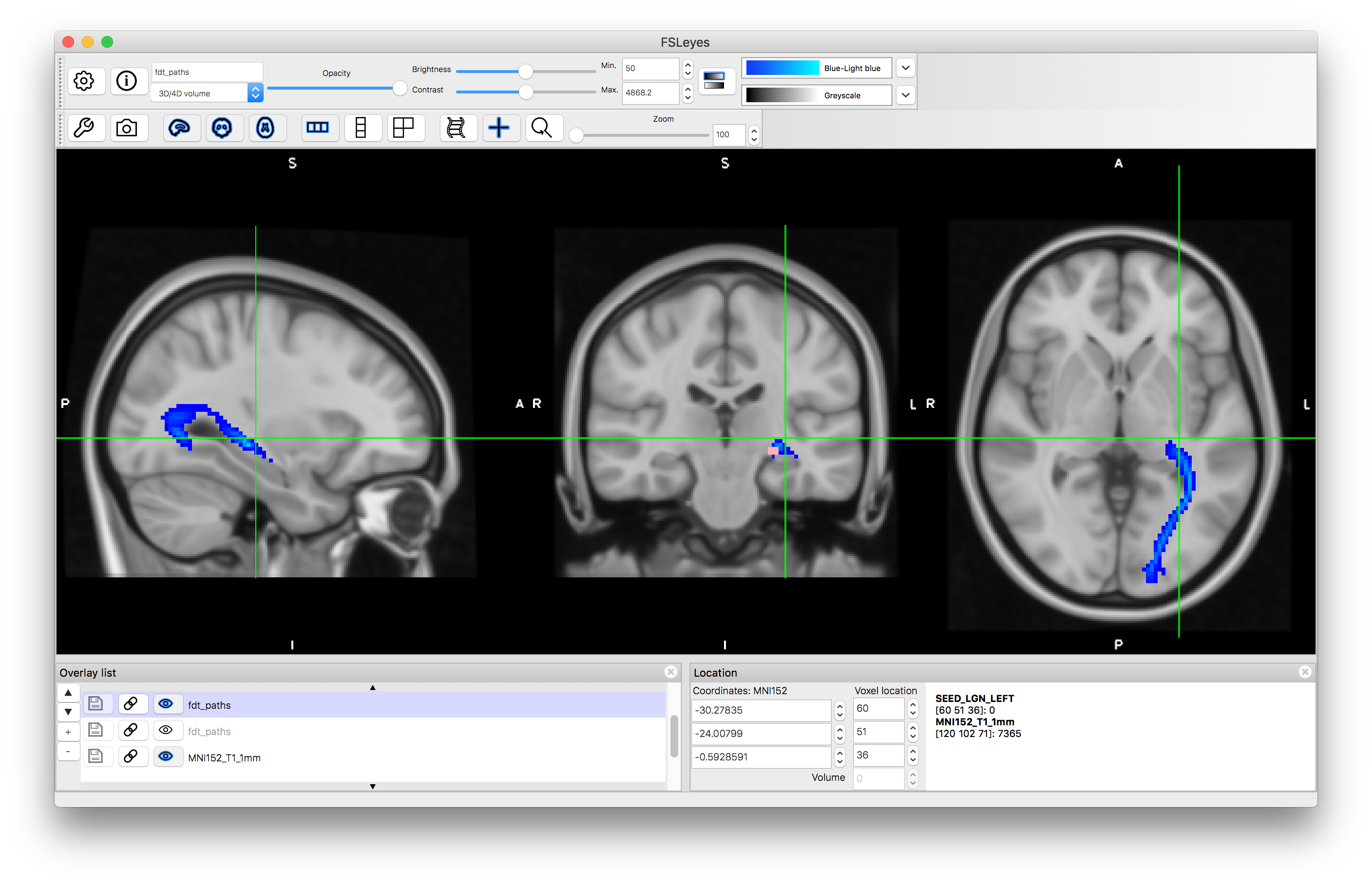
Load the results into a viewer - the image containing the tractography in this case will be called fdt_paths.nii.gz and you can find this in the output directory that you specified. Also load the MNI152_T1_1mm standard brain (using "Add standard") and put this underneath the tractography image in the Overlay list. Apply a colourmap to the tractography result and set its "Min" value to 50.
In this case you will see that there it finds the desired tract as well as other tracts connected to the LGN and some offshoots of the tract of interest. This is expected behaviour for probabilistic tractography, as the random sampling can sometimes result in spurious offshoots into nearby tracts and as we did not specify which direction we wanted it has correctly found the all tracts, in any direction, that connect to the LGN.
Tractography result using LGN seed mask: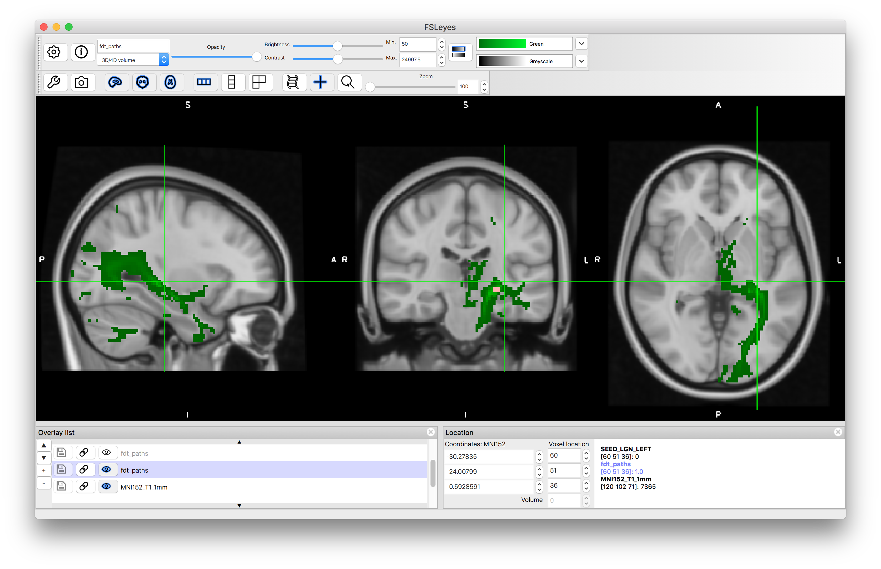
Using waypoint and termination masks
We will now use some additional information to refine the tractography. In particular we will specify a waypoint mask and termination mask. The waypoint mask is used to specify a region that all randomly sampled streamlines must pass through in order to be counted towards the probabilistic result. That is, if a particular streamline does not pass through the waypoint mask then it will be rejected.
The termination mask is used as a stopping criteria, so that whenever a streamline reaches a voxel in the termination mask then it stops there. This avoids tracts continuing on past this region to other parts of the brain.
In this case we will use a mask of V1 (primary visual cortex) called TARGET_V1_LEFT.nii.gz both as a waypoint and a termination mask. This will then isolate only the tracts that connect the LGN to V1 and will prevent these tracts being extended beyond V1 (e.g., excluding real tracts that connect V1 to other parts of the brain). To use these masks you need to run the tractography again, using the above steps but including these additional steps (before pressing "Go"):
- Click on "Waypoint masks" in the "Optional Targets" section and then use the "Add Image" button to select the mask
TARGET_V1_LEFT.nii.gz - Click on the "Termination mask" button in the "Optional Targets" section and use the file browser to select the mask
TARGET_V1_LEFT.nii.gz
Load the result (fdt_paths.nii.gz) from the new output directory on top of the result from before. Give the new result a different colour and set its "Min" value to 50 again. You will see that this result is much more specific and only shows the tract of interest. Also load the mask TARGET_V1_LEFT.nii.gz to see the extent of this mask.
Feel free to experiment with other masks (you can draw them with fsleyes - see online documentation) and other ways of using them. For instance, it is possible to use masks as exclusion masks where any streamline that touches an exclusion mask is rejected. This can, for example, be very helpful to stop tracts crossing between hemispheres by including a mask of the mid-sagittal plane as an exclusion mask.
This example demonstrates how to run probabilistic tractography and how to view the results. Thresholding the results is one of the tricky points in tractography and there is no single way to approach this, as it depends a lot on how the tractography results will be used (e.g., for defining anatomical connectivity matrices; or defining tracts for surgical planning; etc.). The use of waypoint, termination and exclusion masks is extremely useful for isolating specific tracts of interest.