Chapter 5 Example box: Examples of node parcellations

Introduction

The aim of this is to familiarise yourself with the similarities and differences between different parcellations.

In this example we will show different parcellations that are available in the literature. This example is image-based, so you do not need to download any data for this example.

Hard parcellation examples

Data-driven hard parcellation of the cortex into a set of nodes is a highly active research field, with new methods being developed all the time. In this section we will look at three different popular examples of data-driven parcellations.

Yeo parcellation

The first example is from Yeo et al (2011). This is a low-dimensional parcellation into 17 resting state networks (a 7-network version is also available), based on data from 1000 subjects. One key feature of this parcellation is the apparent complexity of cortical regions associated with higher order cognitive processing (association cortices). For example in the middle temporal area, there are several bordering regions with very different patterns of connectivity (i.e., belonging to different large-scale networks).

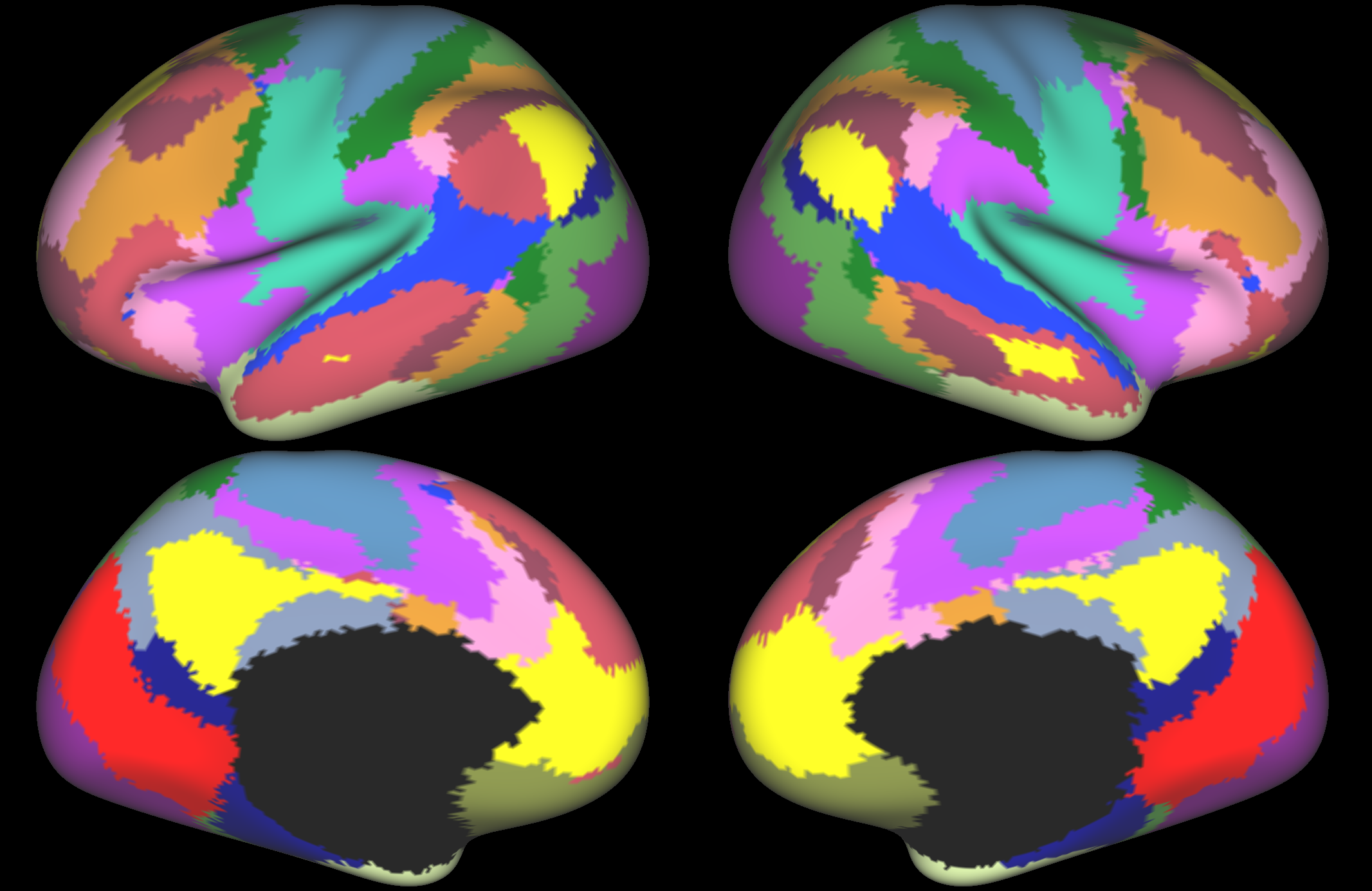
Yeo, B. T. T., Krienen, F. M., Sepulcre, J., Sabuncu, M. R., Lashkari, D., Hollinshead, M., ... Buckner, R. L. (2011). The organization of the human cerebral cortex estimated by intrinsic functional connectivity. Journal of Neurophysiology, 106(3), 1125-1165. https://doi.org/10.1152/jn.00338.2011. Parcellation available to download from: https://surfer.nmr.mgh.harvard.edu/fswiki/CorticalParcellation_Yeo2011.

Glasser parcellation

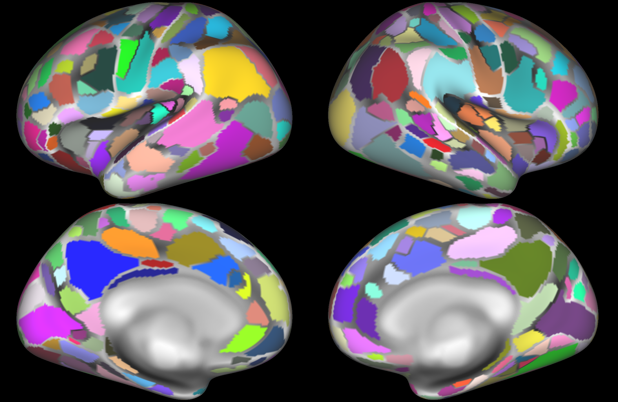
This example, from Glasser et al (2016), parcellates the cortical surface into 360 nodes based on data from 210 subjects. A detailed anatomical description of the functional and structural features of these nodes is included in the publication. A key feature of this parcellation is the fact that multiple modalities were used to identify node boundaries, including myelin and cortical thickness maps, as well as task-fMRI activation and functional connectivity. This led to the identification of multiple novel brain areas, and demonstrated atypical topological organisation of certain brain regions (including the frontal eye fields) in some individuals.

Glasser, M. F., Coalson, T. S., Robinson, E. C., Hacker, C. D., Harwell, J., Yacoub, E., ... Van Essen, D. C. (2016). A multi-modal parcellation of human cerebral cortex. Nature, 536(7615), 171-178. https://doi.org/10.1038/nature18933. Parcellation available to download from: https://balsa.wustl.edu/file/show/3VLx.

Gordon parcellation

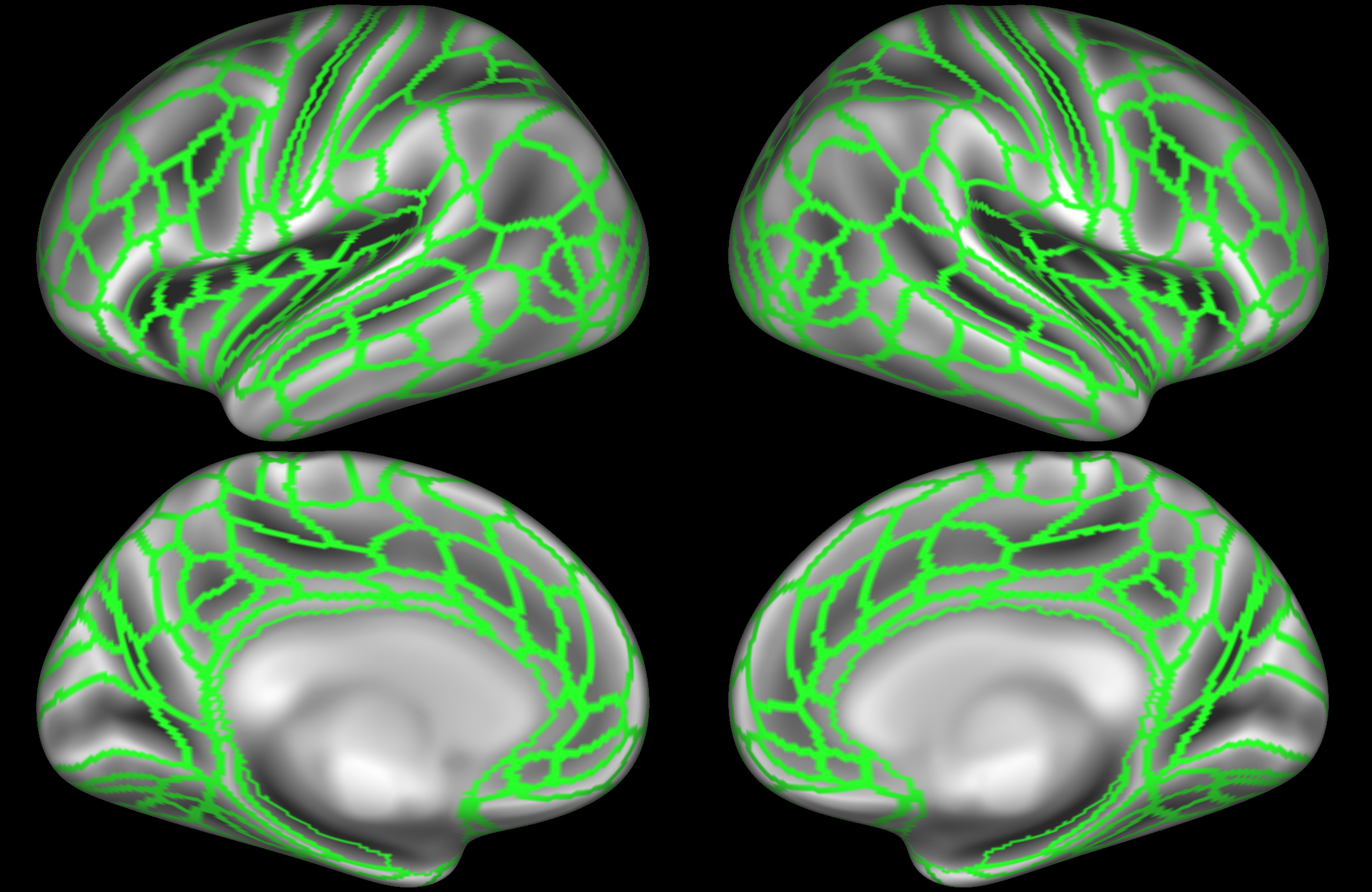
The last example, from Gordon et al (2016), parcellated the brain into 422 nodes based on data from 120 subjects. A key feature of this parcellation is that it is driven by a boundary map of resting state functional connectivity. This boundary map shows transition areas, where the whole-brain functional connectivity pattern changes rapidly from one location to a neighbouring location. Boundary regions with rapid transitions were excluded from the parcellation (i.e., some surface locations are not part of any node). As a result, the parcels are found to have high homogeneity compared with other parcellation approaches.

Gordon, E. M., Laumann, T. O., Adeyemo, B., Huckins, J. F., Kelley, W. M., & Petersen, S. E. (2016). Generation and Evaluation of a Cortical Area Parcellation from Resting-State Correlations. Cerebral Cortex , 26(1), 288-303. https://doi.org/10.1093/cercor/bhu239. Parcellation available to download from: http://www.nil.wustl.edu/labs/petersen/Resources.html.

ICA dimensionality example

One of the most commonly used soft parcellation methods is Independent Component Analysis (ICA). If the aim is to perform a subsequent node-based analysis, it is common to set the ICA decomposition dimensionality between 50 and 500, depending on the number of subjects and the number of timepoints per subject. Increasing the dimensionality results in components being split across multiple nodes. The aim of this example is to show an example of the type of splitting seen using an example dataset.

In this example we look at data from 820 subjects in the Human Connectome Project. Concatenated group ICA was performed using the same data, at multiple dimensionalities (50, 200, 400 nodes). In the figures below, we show how the brain areas of two large-scale resting state networks (the default mode network and the dorsal attention network) are split into nodes depending on the dimensionality. This is an example of how the dimensionality interacts with the decomposition in order to give you some intuition. However, it should be noted that the way components are split will differ depending on the dataset.

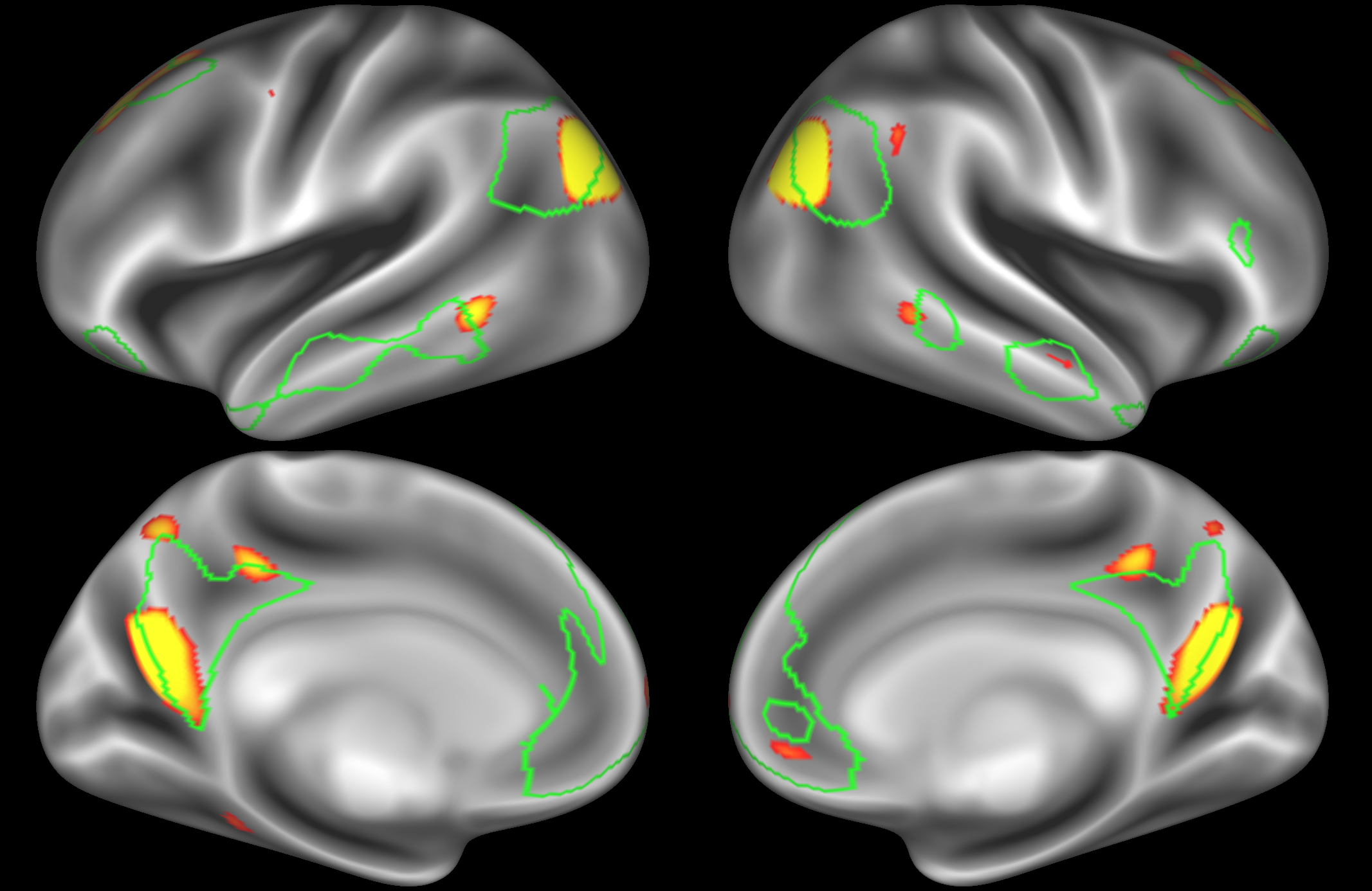
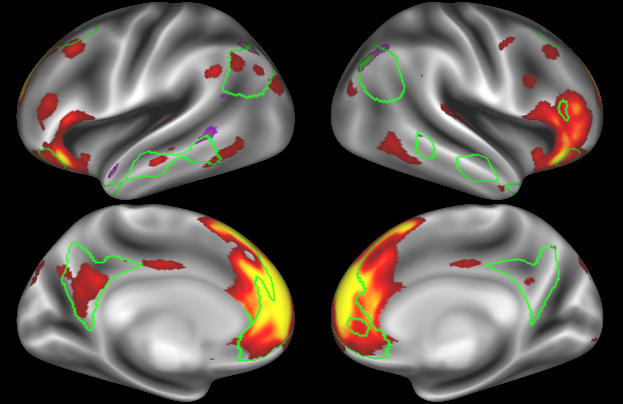
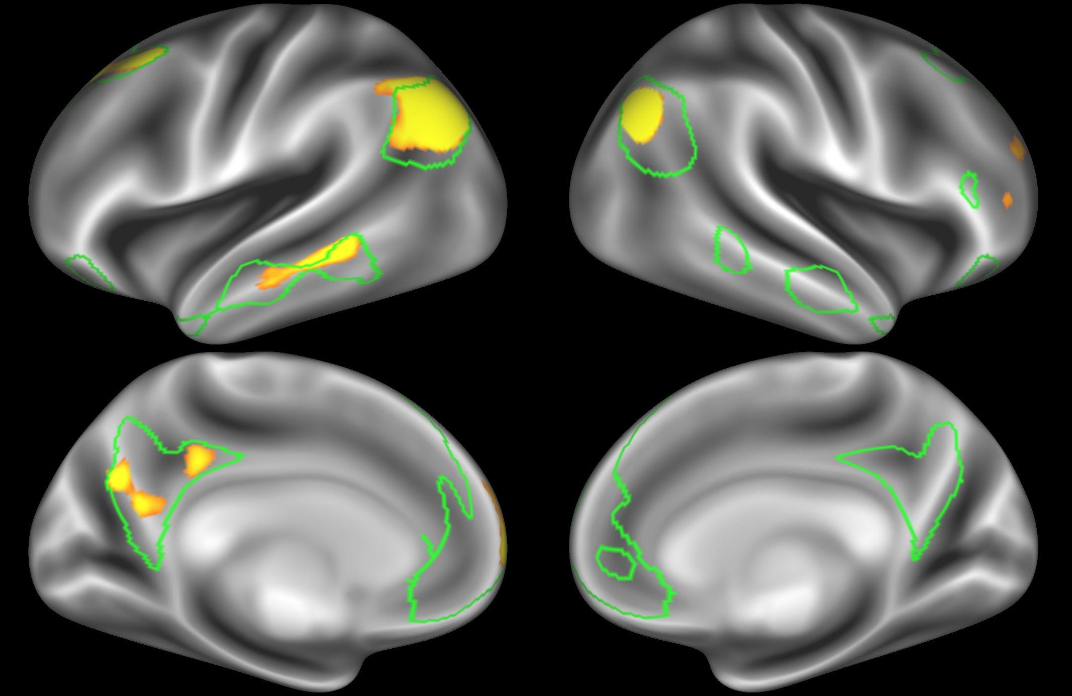
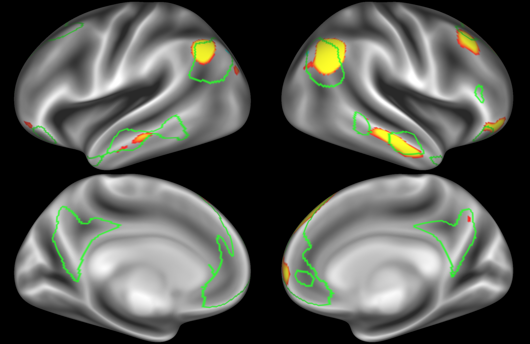
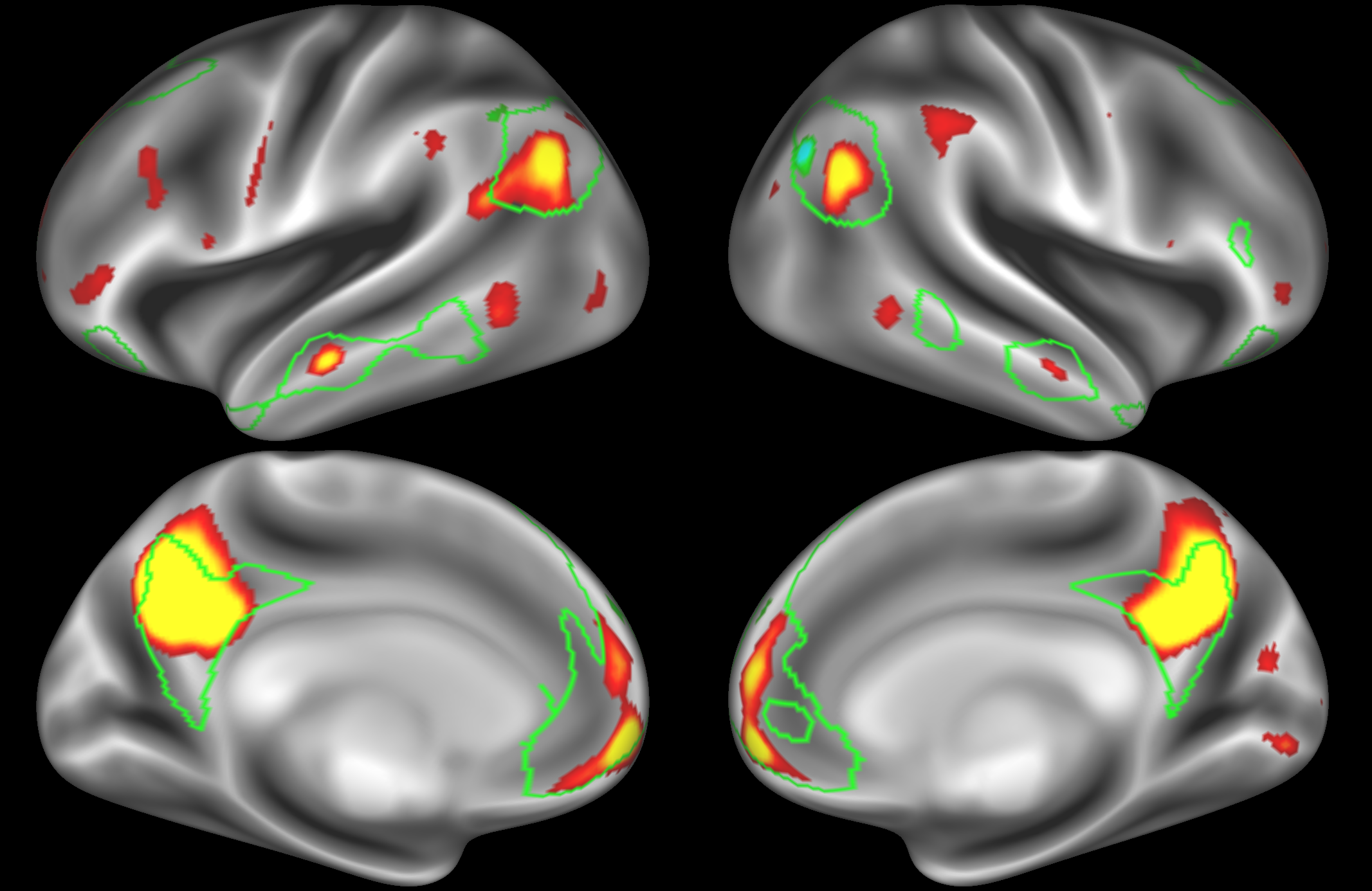
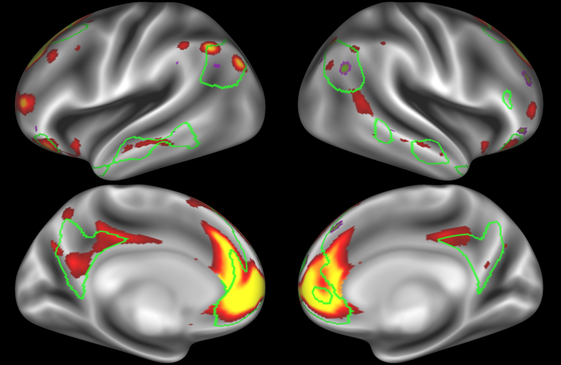
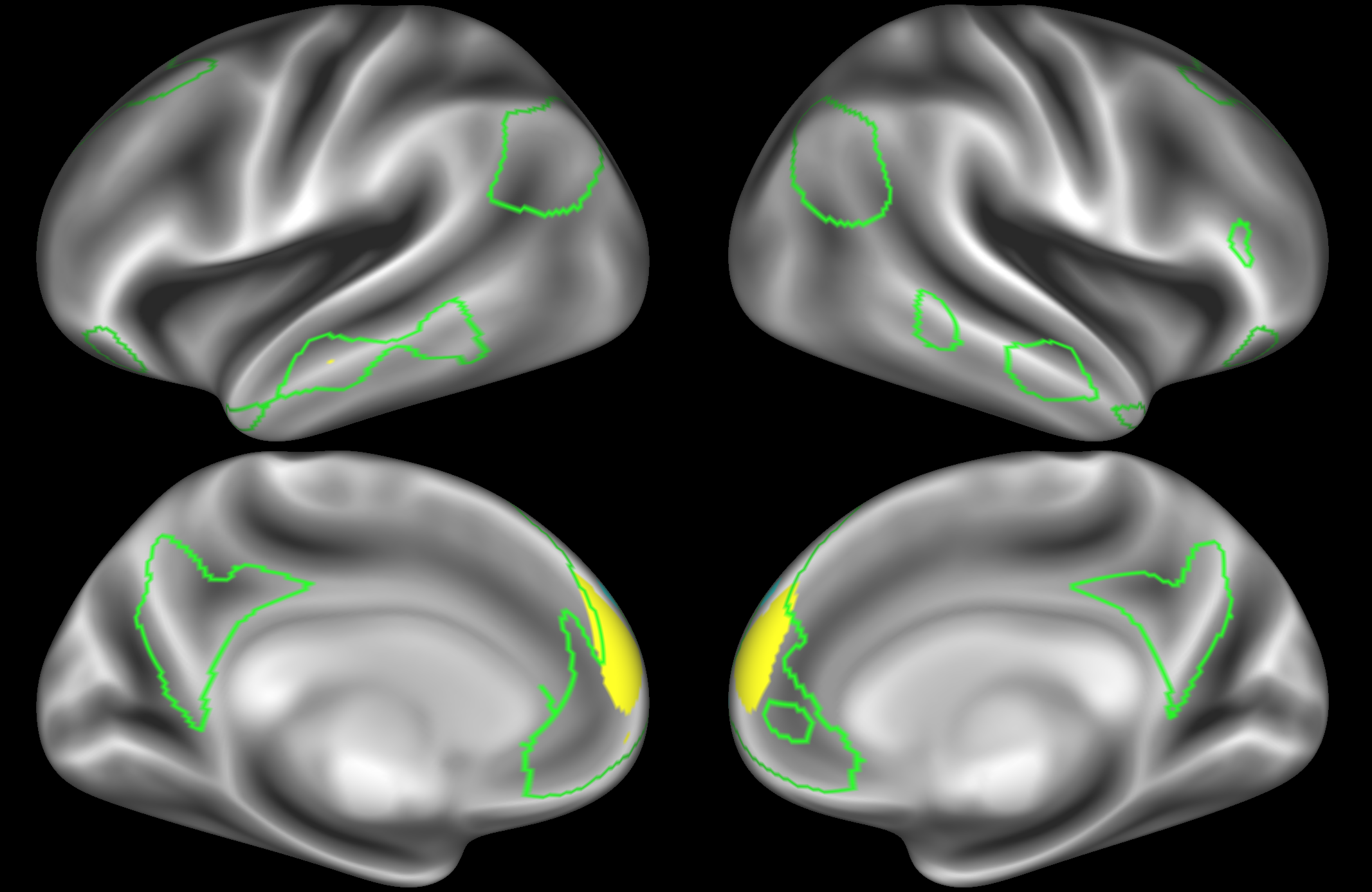
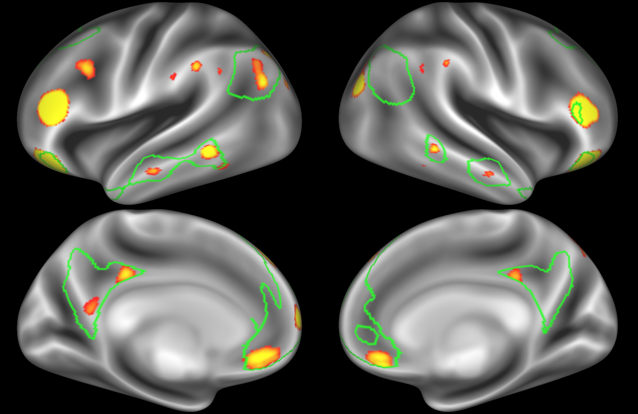
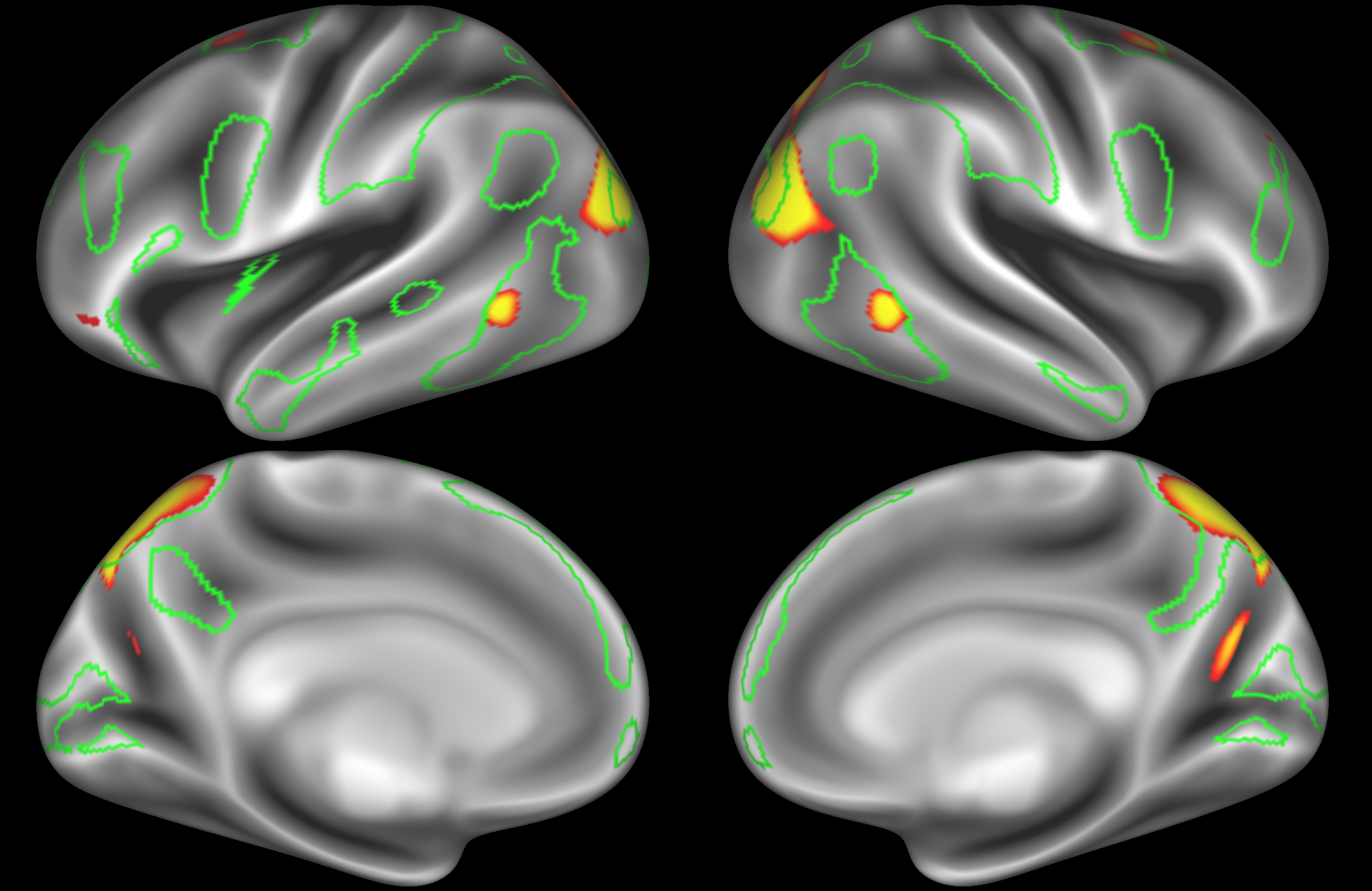
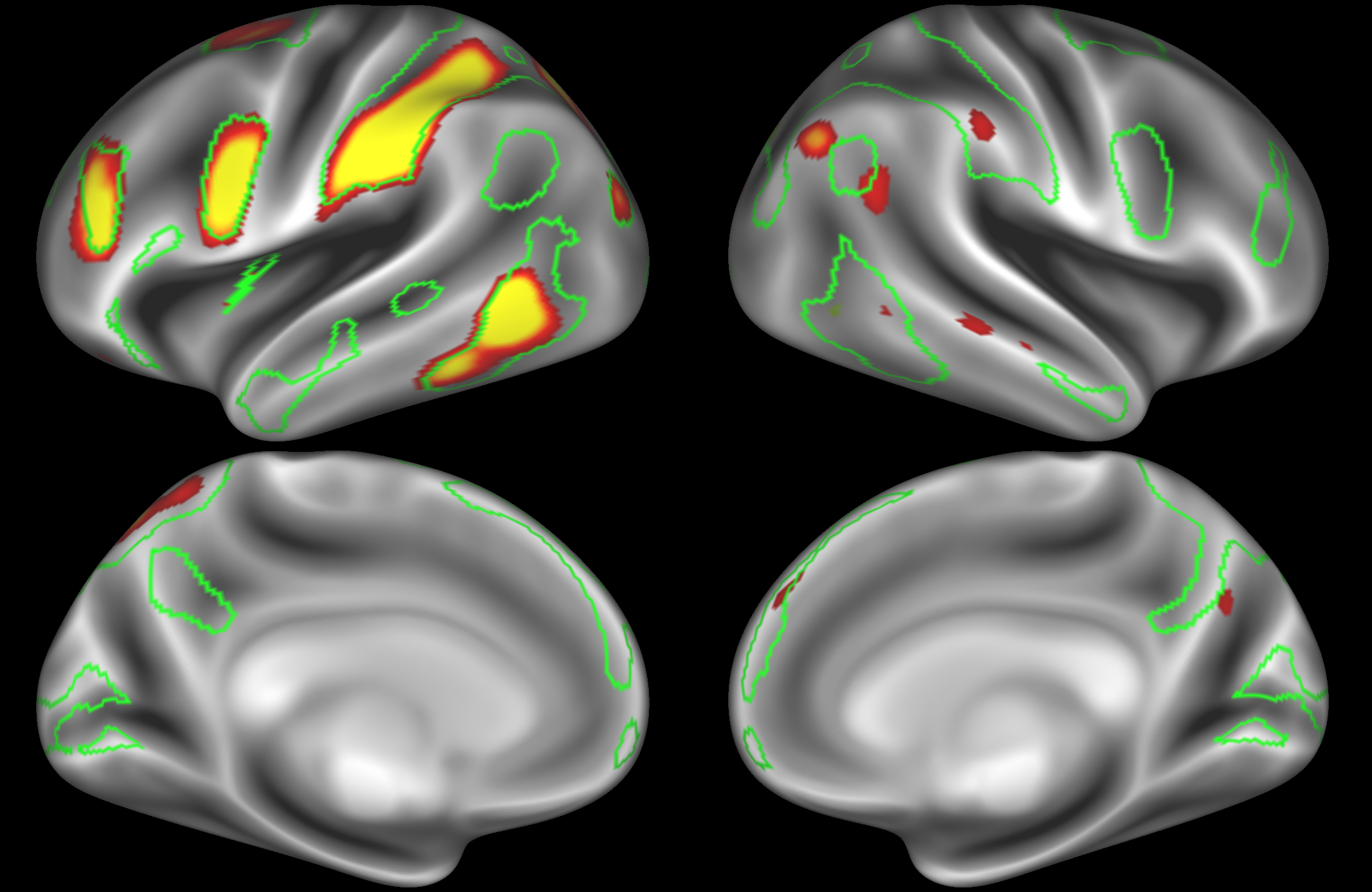
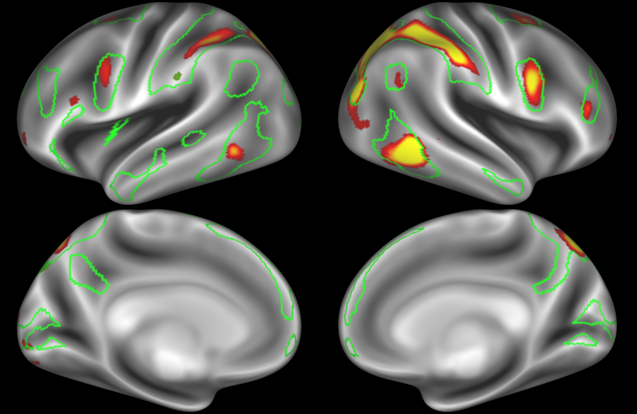
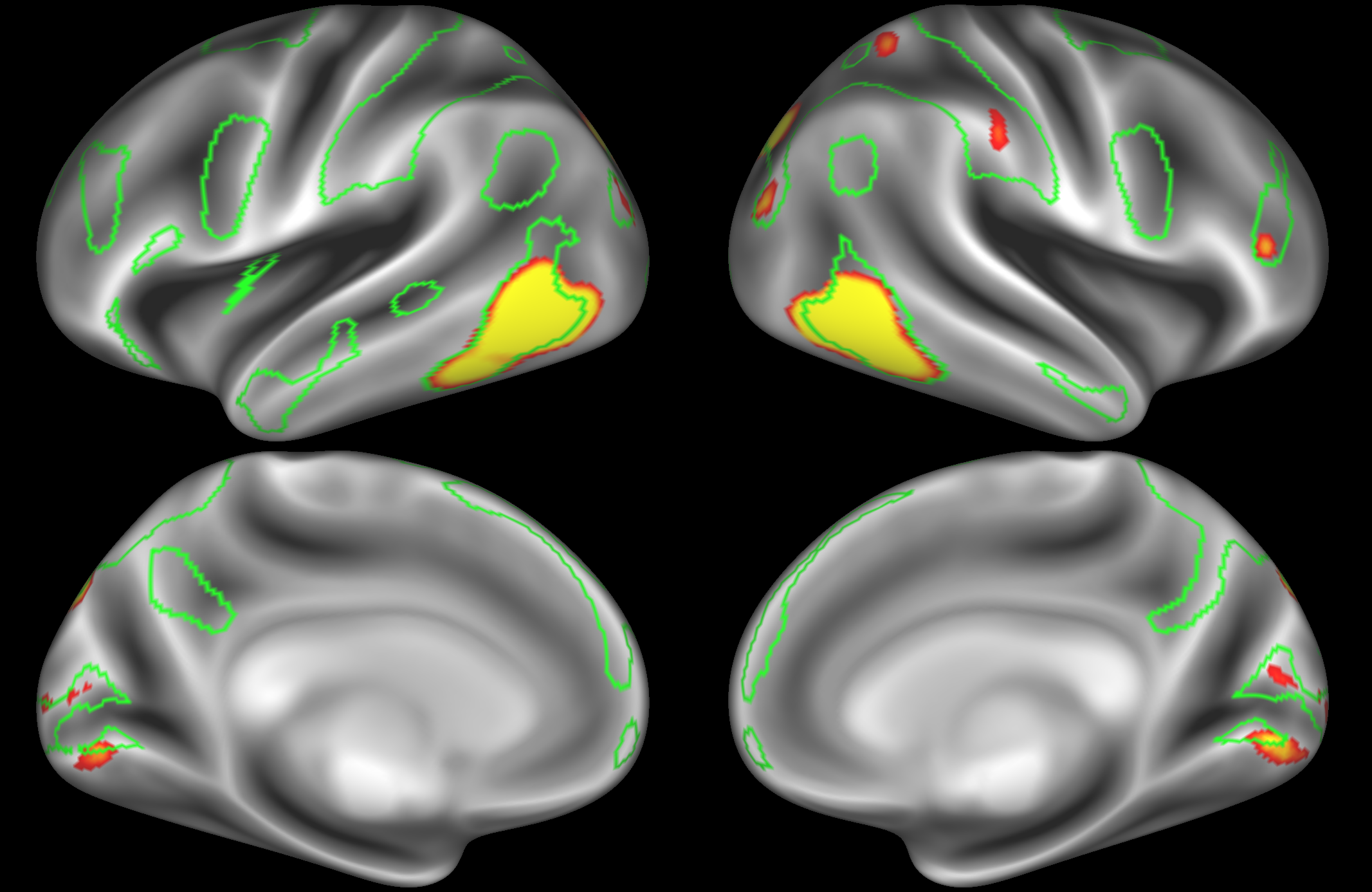
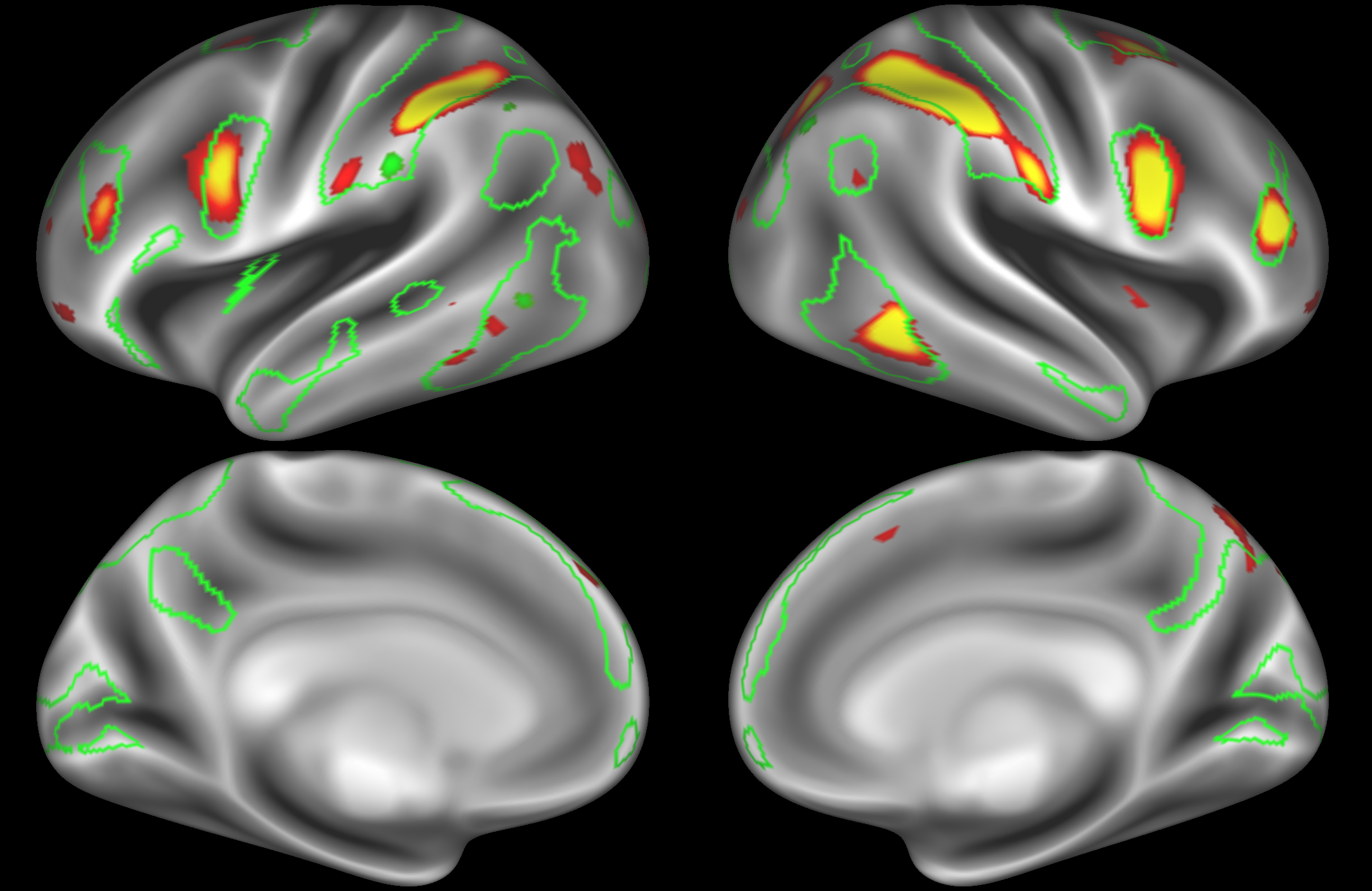
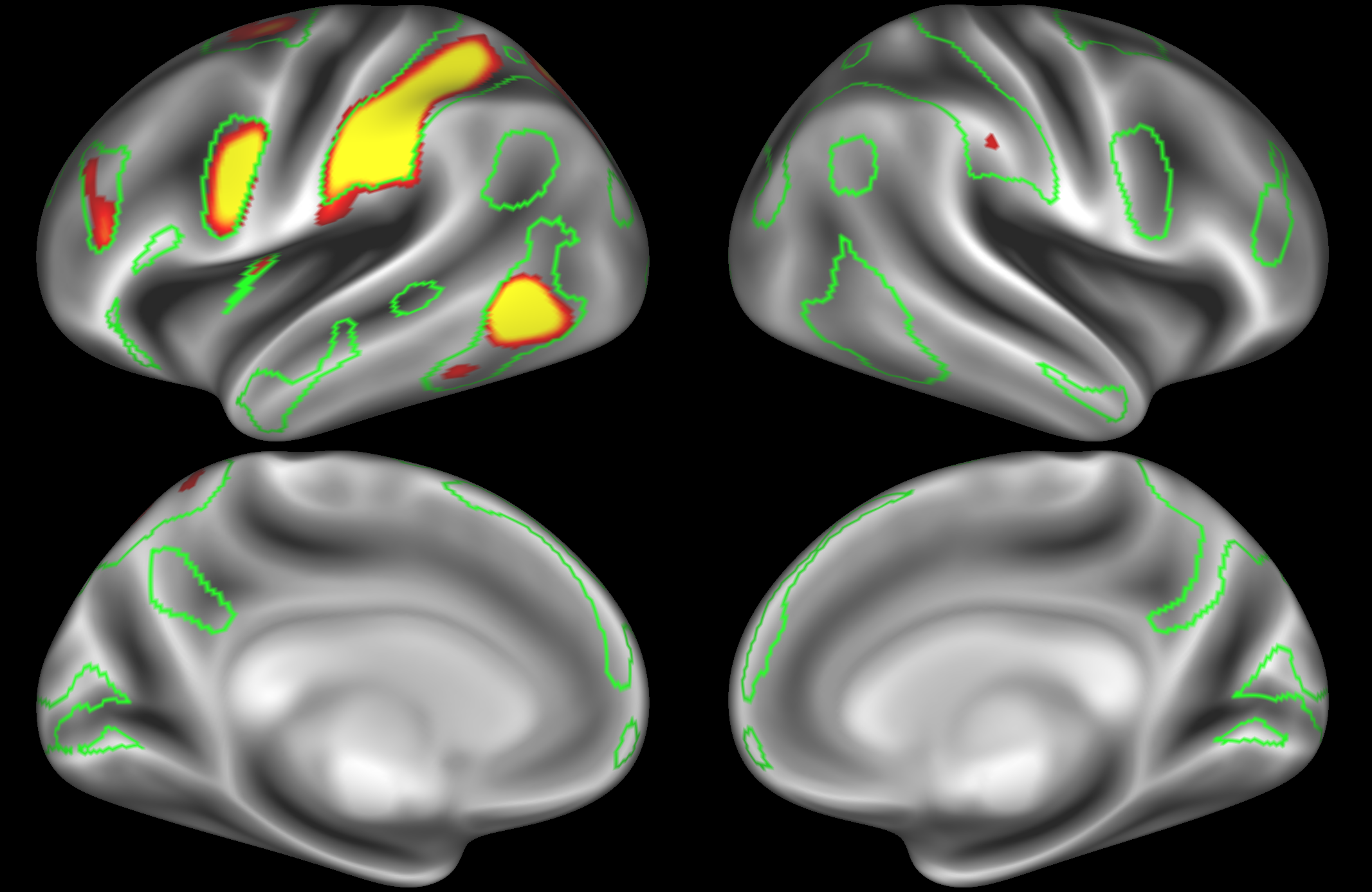
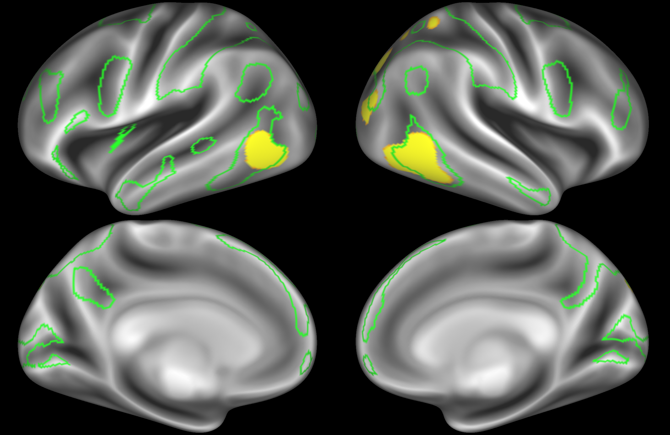
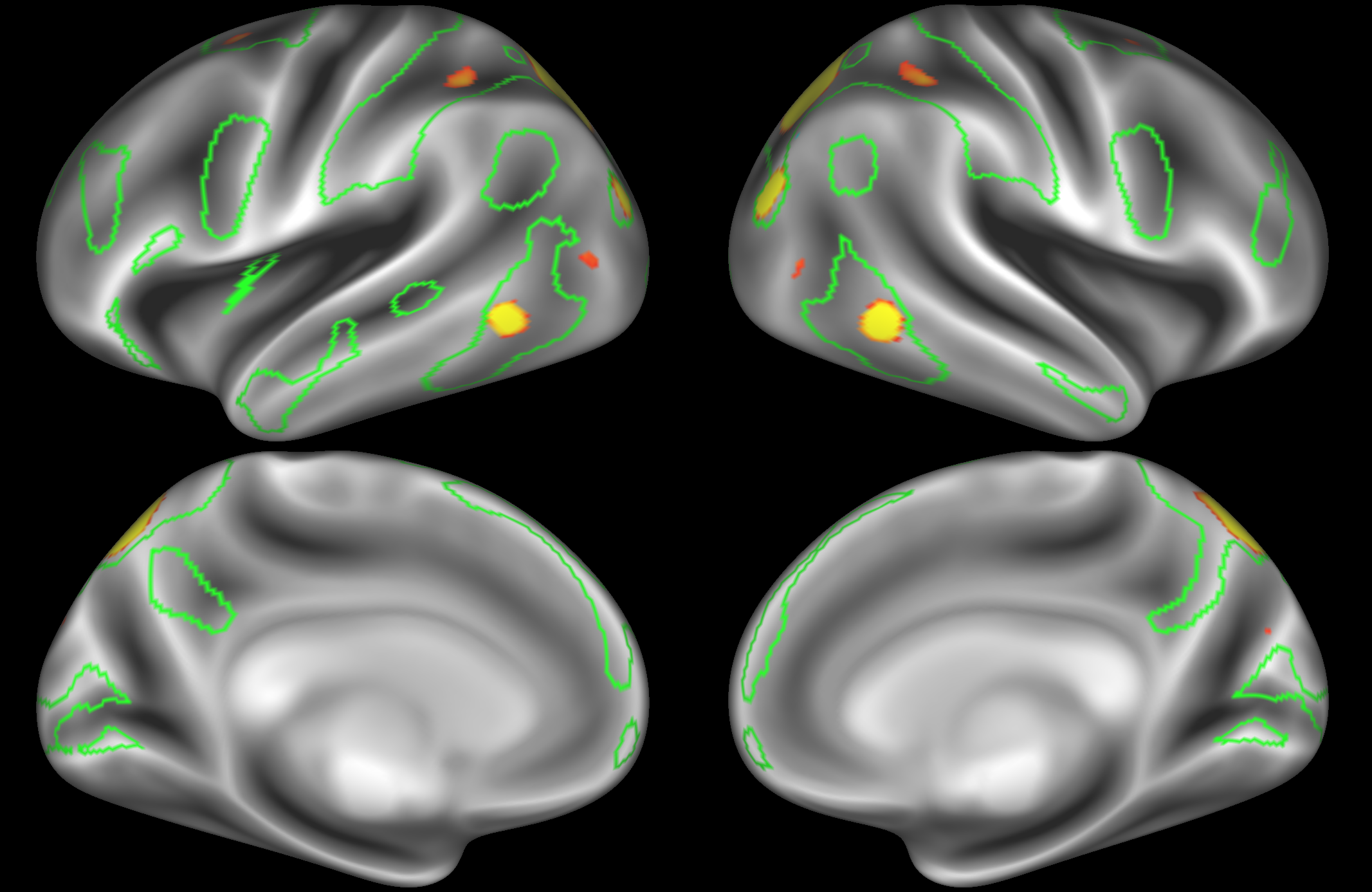
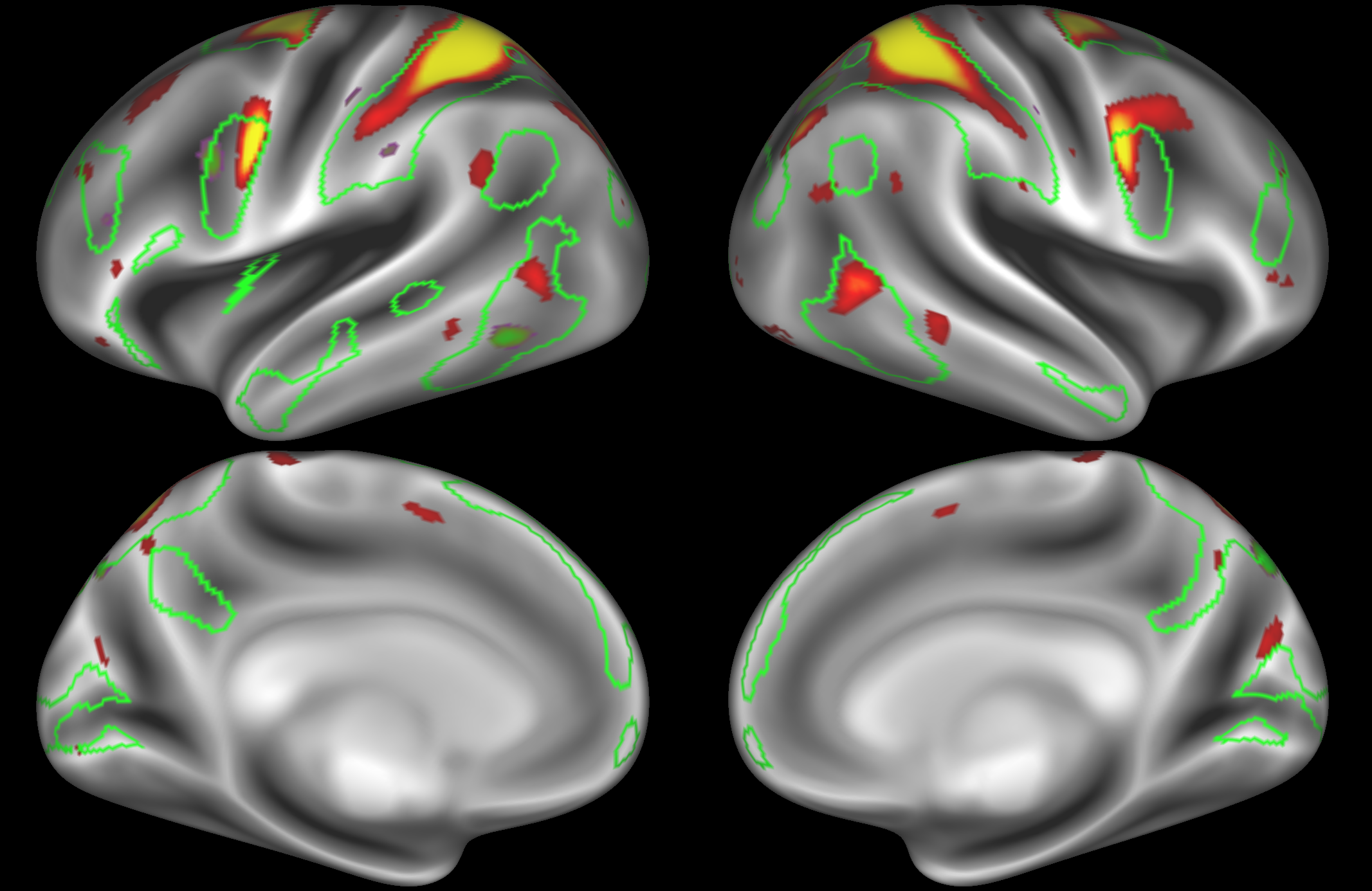
Default mode network

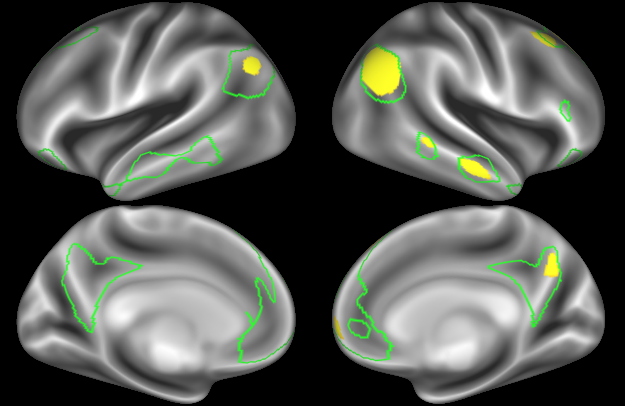
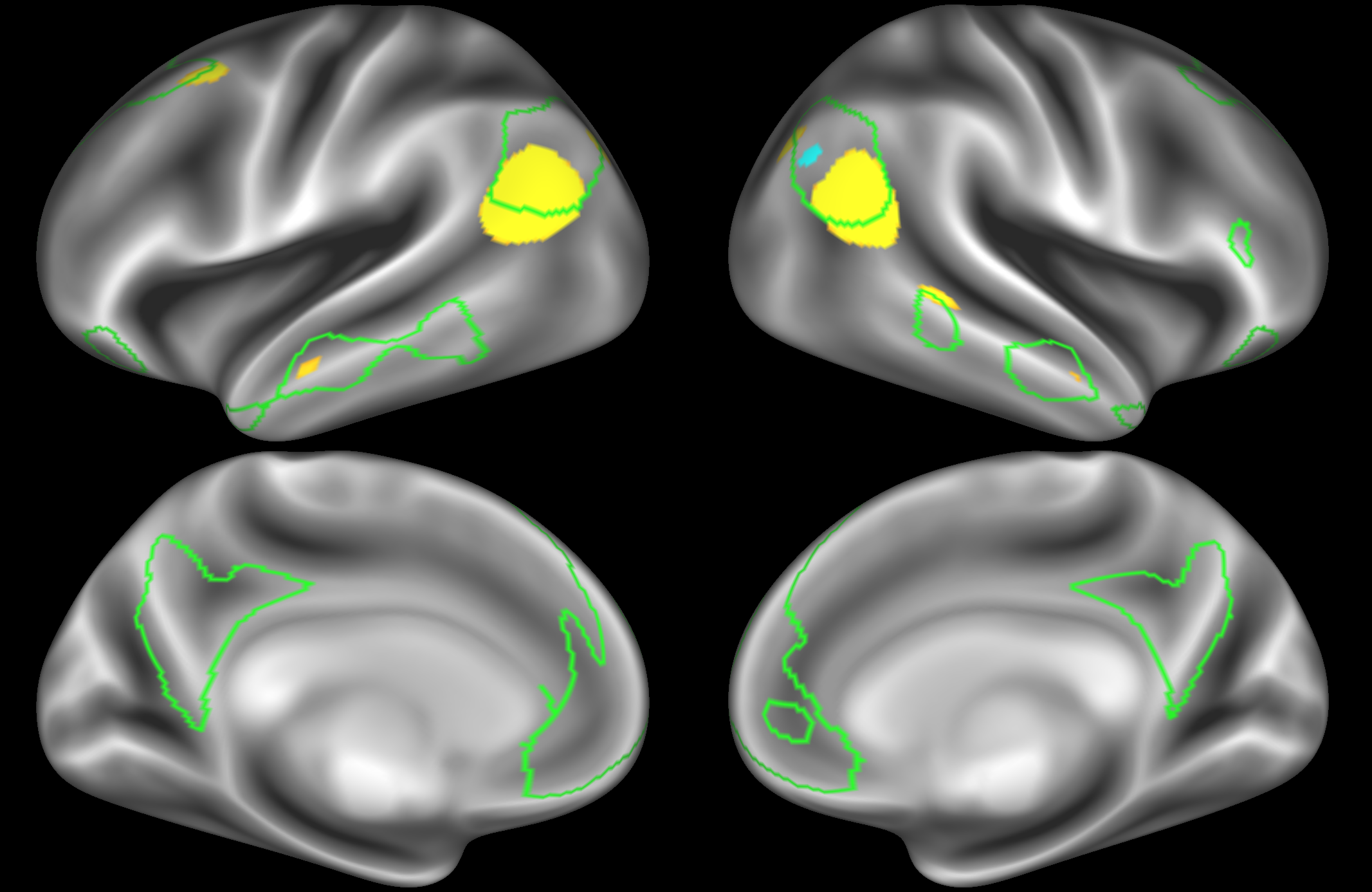
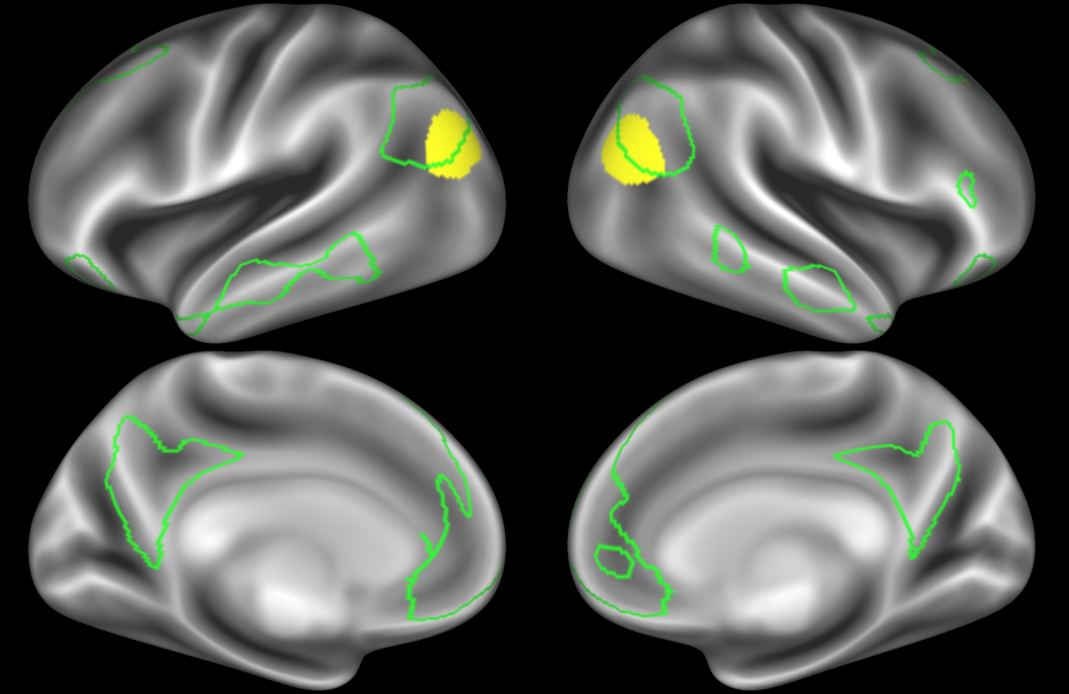
In the example below, the outline of the DMN resting state network is shown in lime green, and any nodes that showed significant overlap with the lime green regions are displayed. At a dimensionality of 50 nodes this RSN was split into 4 nodes, at d=200 it was split into 7 nodes, and at d=400 it was split into 8 nodes. Each of these is shown in the figures below. The figures show the nodes on the cortical surface, and are thresholded to help with visualisation.

ICA 50 nodes:

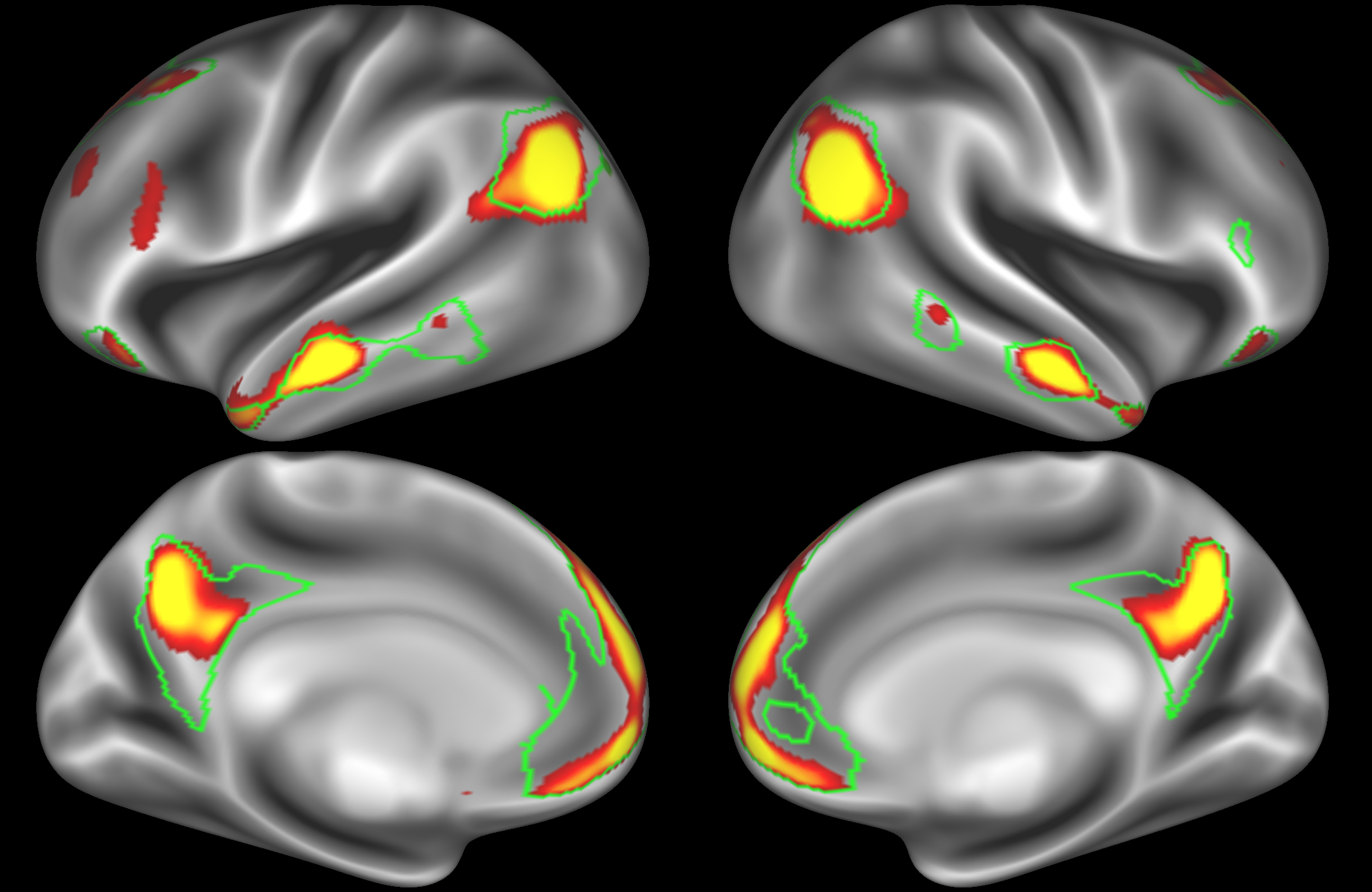
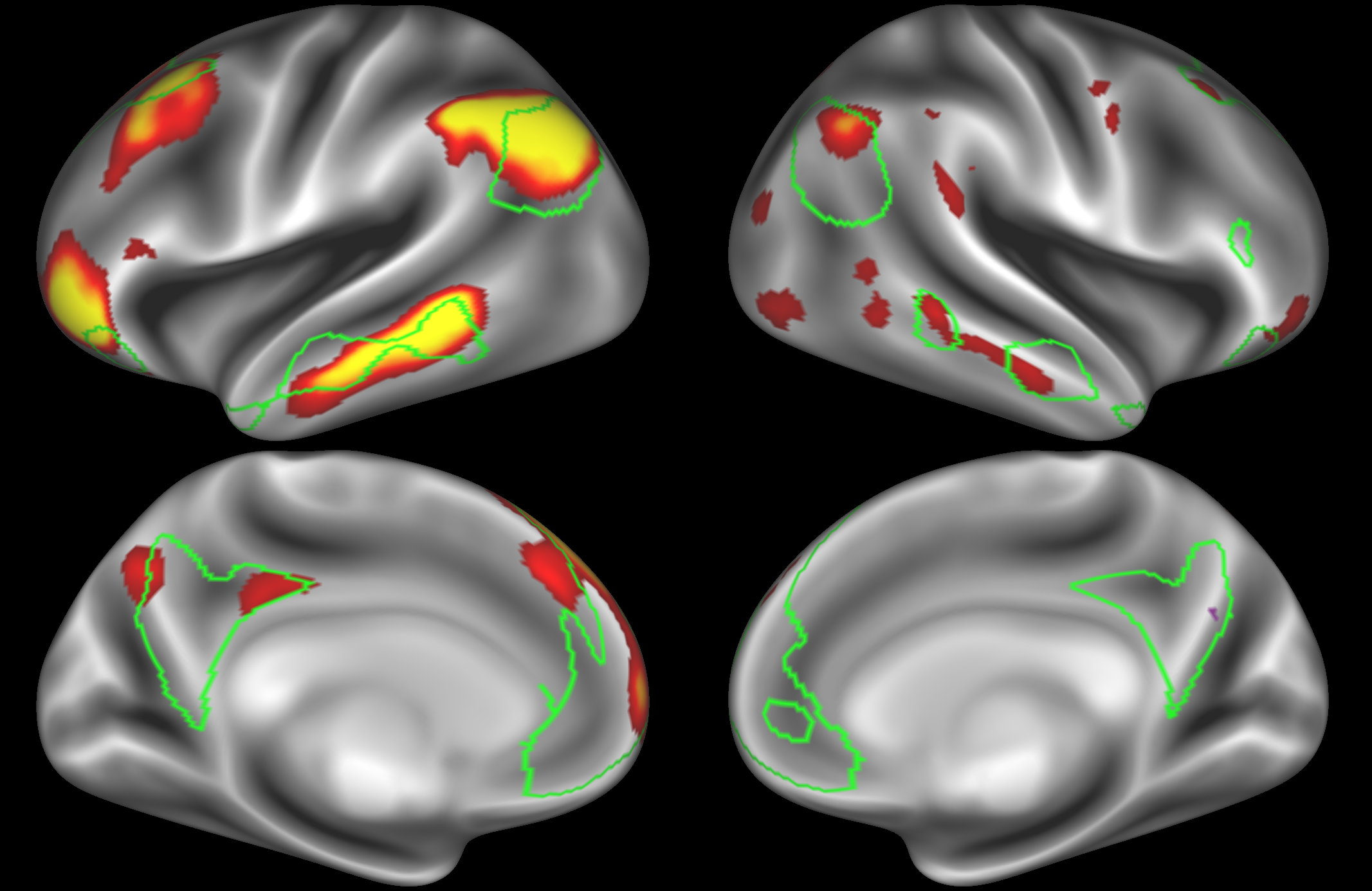
Note how the posterior cingulate/ precuneous region is split across the two nodes on the top left and bottom left.

ICA 200 nodes:

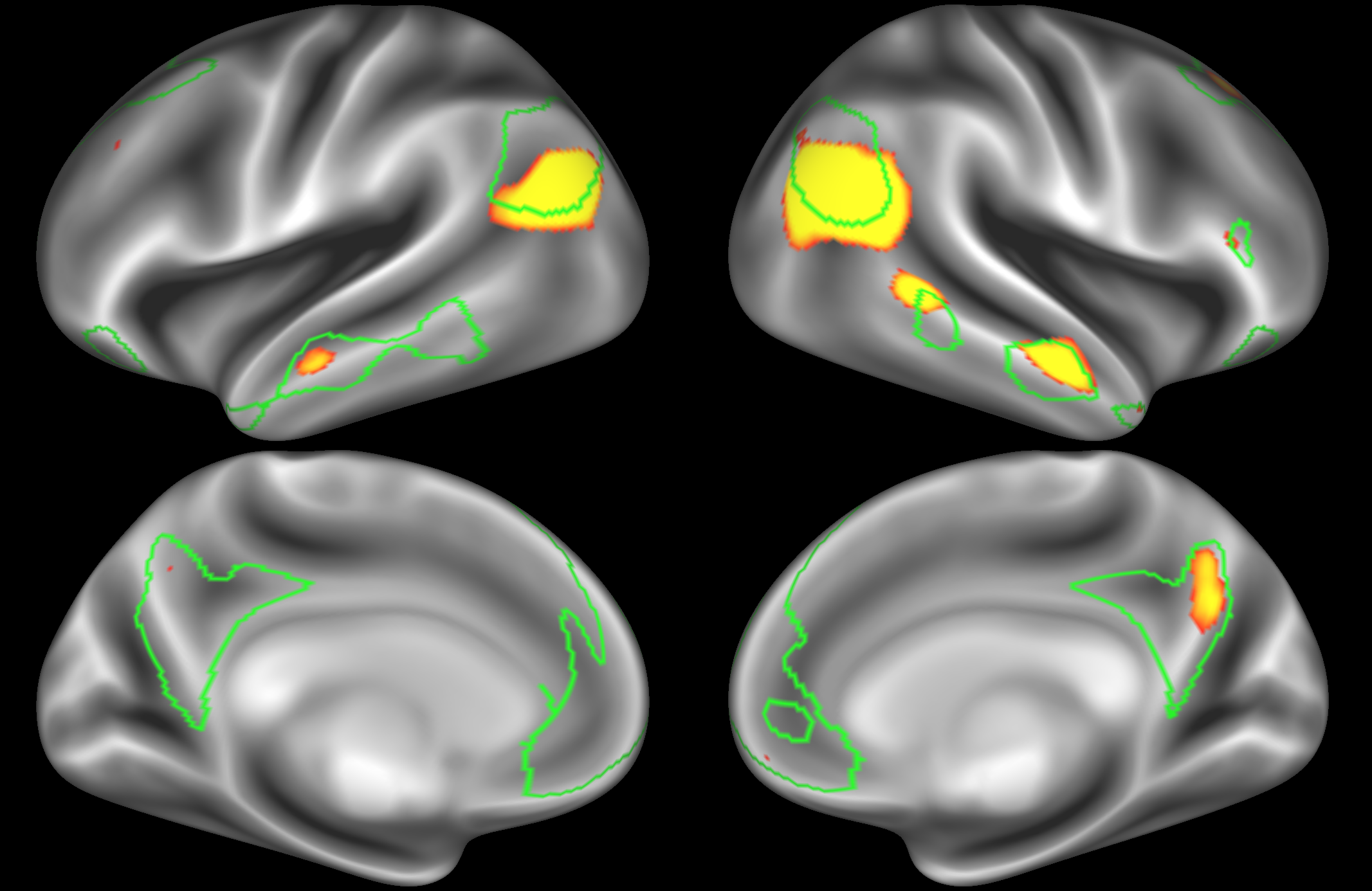
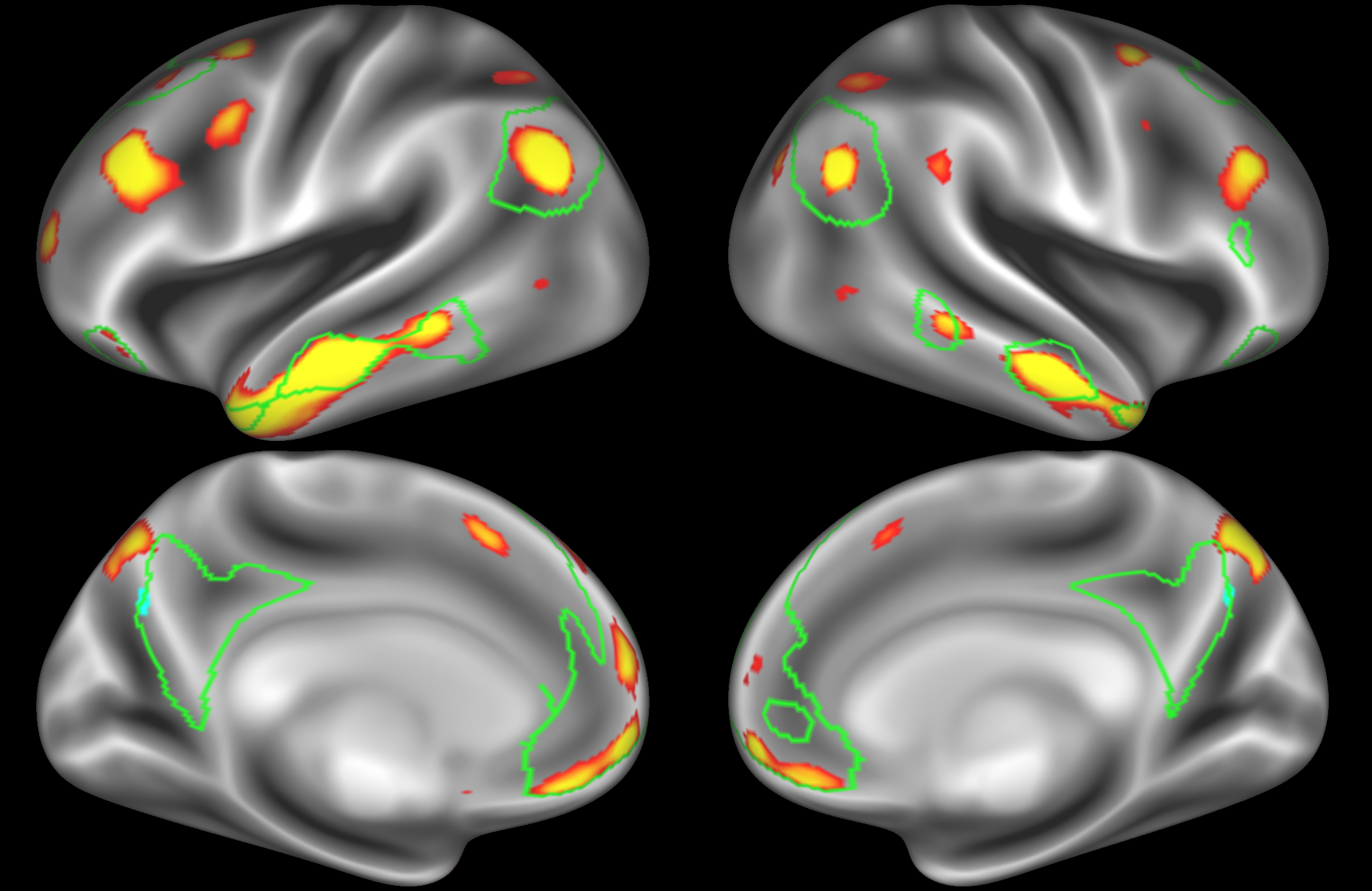
At this dimensionality it is clear that the DMN is broken down into nodes that each contain bilateral subregions of the resting state network.

ICA 400 nodes:

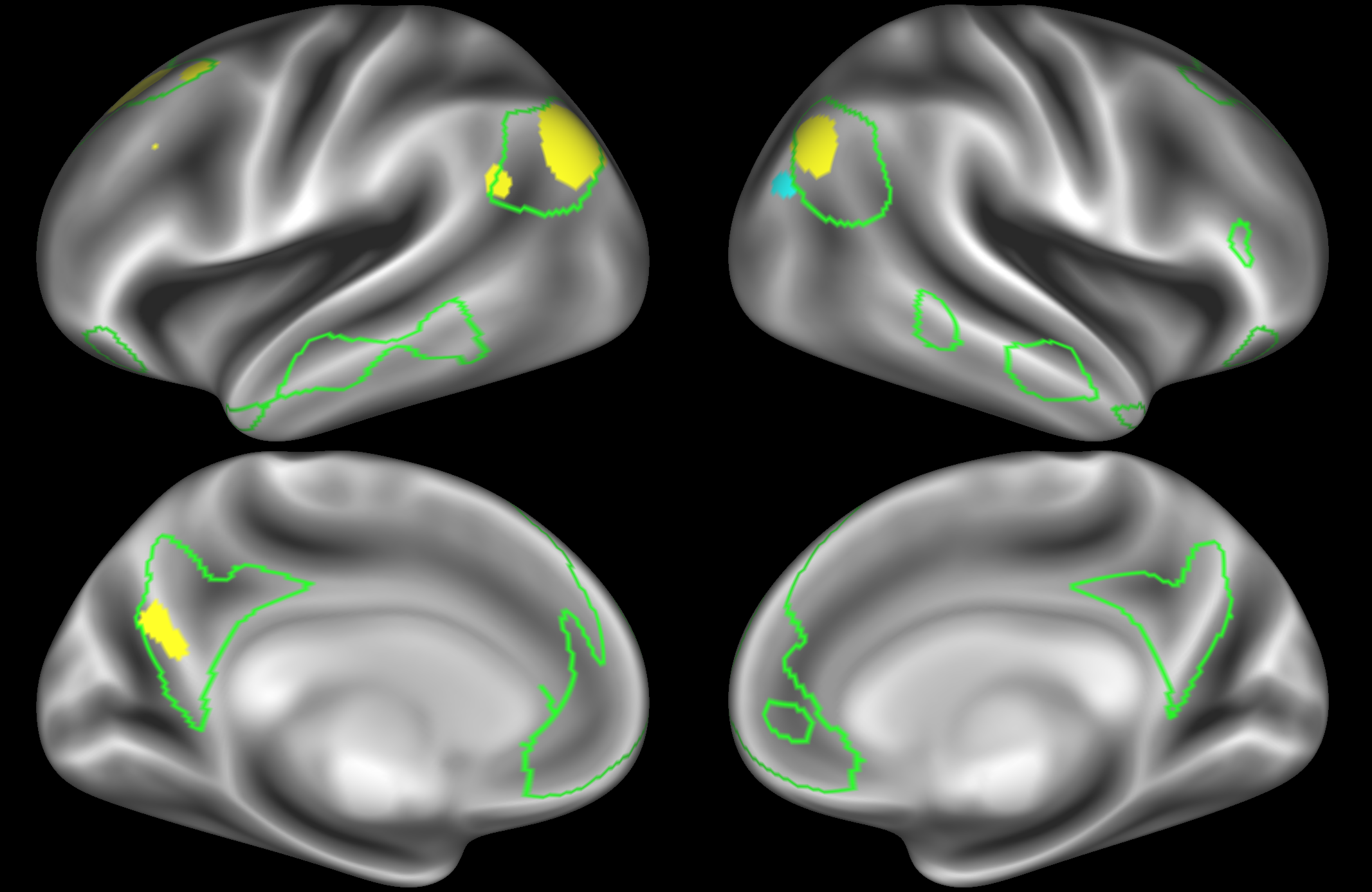
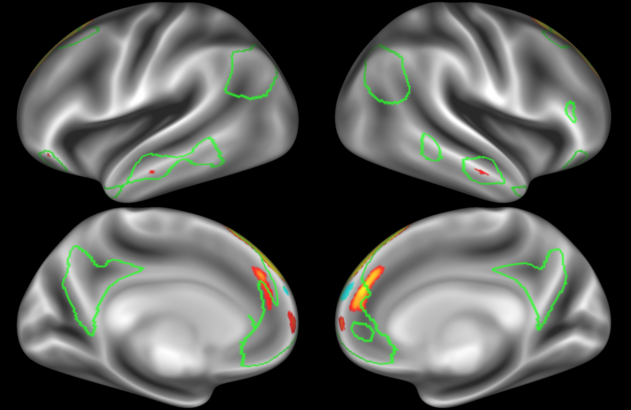
At this high dimensionality, the resting state networks gets further split into smaller sub-regions. Note that there are four different nodes that represent some part of the inferior parietal lobule (shown in the top 3 images on the left and the second image on the right), which may be suggestive of overspliting.

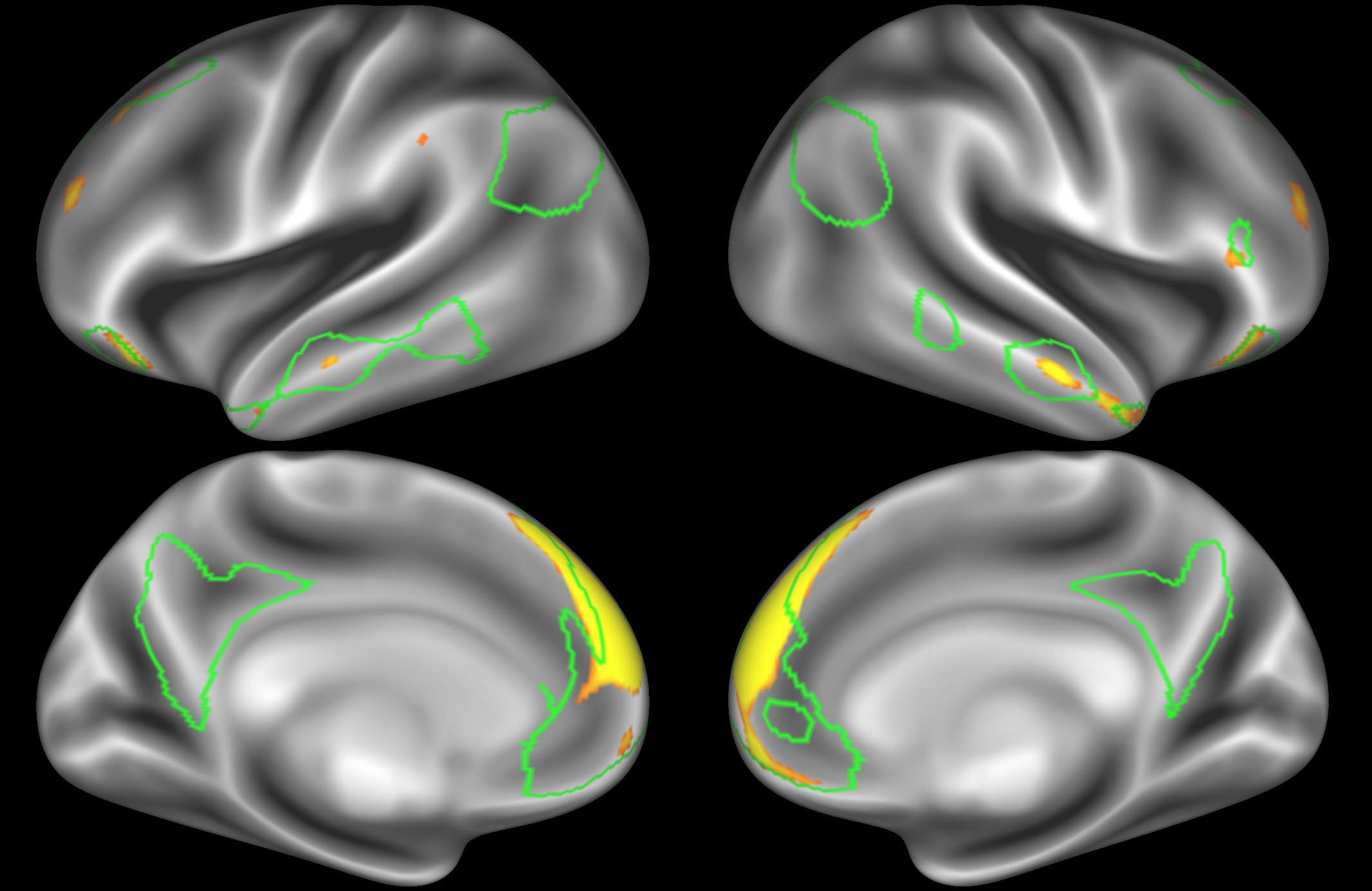
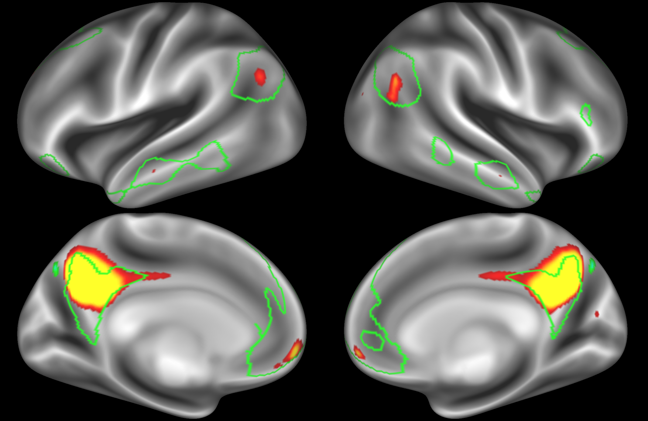
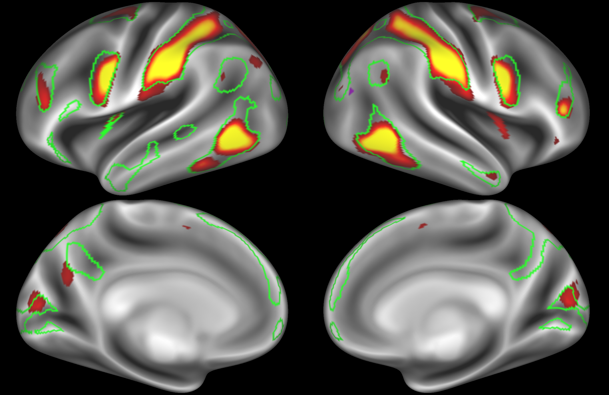
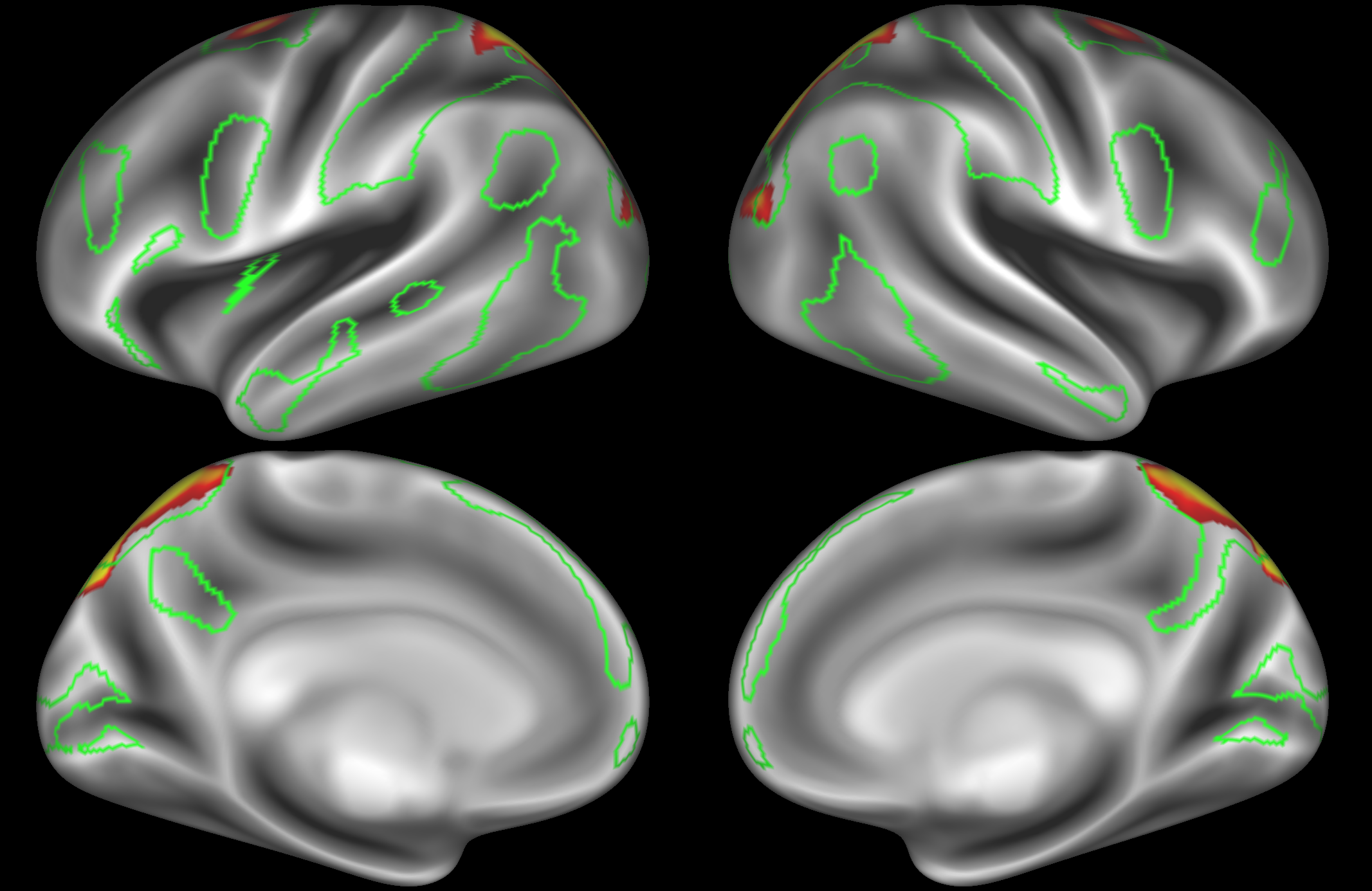
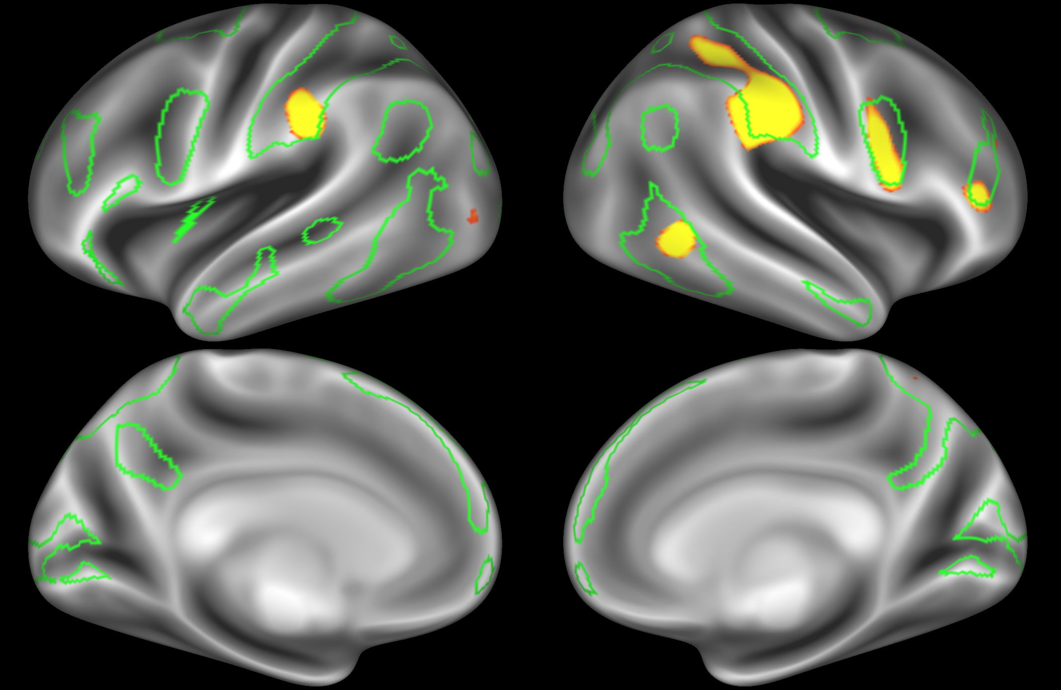
Dorsal attention network

In the example below, the outline of the DAN resting state network is shown in lime green, and any nodes that showed significant overlap with the lime green regions are displayed. At a dimensionality of 50 nodes this RSN was split into 2 nodes, at d=200 it was split into 5 nodes, and at d=400 it was split into 6 nodes. Each of these is shown in the figures below. The figures show the nodes on the cortical surface, and are thresholded to help with visualisation.

ICA 50 nodes:

At this relatively low dimensionality, the DAN is split into two separate nodes.

ICA 200 nodes:

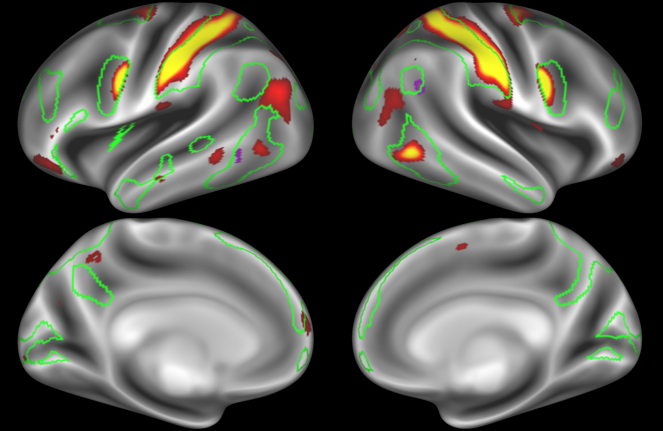
Here the DAN is split into multiple nodes including a left-lateralised and a right-lateralised version of the network (top two images).

ICA 400 nodes:

Note the similarities and differences between the 200 and 400 parcellation. For example, the left and right lateralised nodes are still present (top right and middle left). It is also noticeable how the middle temporal sub-region is split across nodes.

Data credits

Literature parcellations are shown from:

This example includes data from the Human Connectome project (https://www.humanconnectome.org/).