Illustration

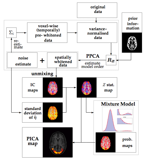
Figure 4: Schematic illustration of the analysis steps involved in estimating the PICA model.

The individual steps that constitute the Probabilistic Independent Component Analysis are illustrated in figure 4. The de-meaned original data are first temporally pre-whitened using knowledge about the noise covariance $\Sigma$$_i$ at each voxel location. The covariance of the data is calculated from the data after normalization of the voxel-wise standard deviation. In the case where spatial information is available, this is encoded in the estimation of the sample covariance matrix $R$$_{\mbox{\protect\boldmath $x$}}$. This is used as part of the probabilistic PCA steps to infer upon the unknown number of sources contained in the data, which will provide us with an estimate of the noise and a set of spatially whitened observations. We can re-estimate $\Sigma$$_i$ from the residuals and iterate the entire cycle. In practice, the output results do not suggest a strong dependency on the form of $\Sigma$ and preliminary results suggest that it is sufficient to iterate these steps only once. From the spatially whitened observations, the individual component maps are estimated using the fixed point iteration scheme (equation 13). These maps are separately transformed to $Z$ scores using the estimated standard deviation of the noise. In contrast to raw IC estimates, the $Z$ score maps depend on the amount of variability explained by the entire decomposition at each voxel location. Finally, Gaussian Mixture Models are fitted to the individual $Z$ maps in order to infer voxel locations that are significantly modulated by the associated time course in order to allow for meaningful thresholding of the $Z$ images.