Theorem:
The two-level model specified by equations 1 and 6 is fully equivalent to the single-level model specified by equation 4 in terms of both modelling and estimation when
That is, the second-level covariance is set as the sum of the group-covariance from the single-level model and the first-level parameter covariance from the two-level model.
Proof:
We employ the Sherman-Morrison-Woodbury formula (equation 17 from the appendix)
to write
![]() as
as
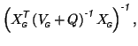
and let
which is the covariance estimate for the
![]() s, from
equation 5.
s, from
equation 5.
Then
Inserting this into equation 8 gives
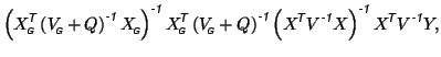 |
|||
 |
which becomes equivalent to equation 9 if
|
|
For this choice of
![]() , the group-level parameter estimates can be written as
, the group-level parameter estimates can be written as
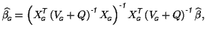
that is, they become a function of the first-level parameter estimates
![]() and their associated covariances
and their associated covariances
![]() only.
only.
Note that by simply applying this theorem multiple times, these
results extend to any multi-level GLM. For example, one can calculate
parameter estimates for groups of groups using a multi-level approach
by only keeping track of parameter estimates and associated
covariances at each level. Note also that parts of this proof can
simply be obtained by characterising the necessary conditions on
sufficient statistics for
![]() [16].
[16].
