Single Tapers

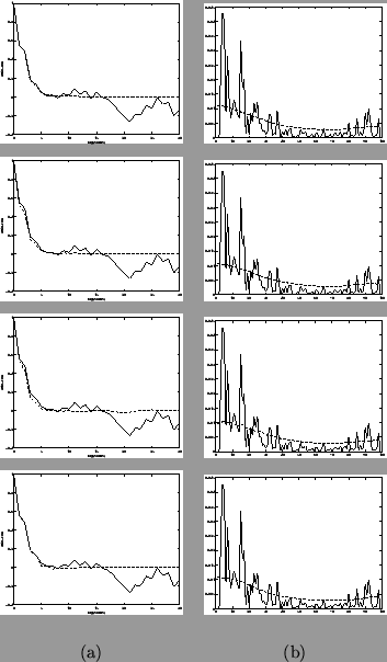
A standard approach to taking raw estimates of the autocorrelation or equivalently of the spectral density is to window the raw time series prior to taking a Fourier Transform. This down-weights points at either end of the time series, reducing leakage due to end effects (Bracewell, 1978). Equivalently the raw autocorrelation estimate can be tapered such that it is downweighted at high lags. Intuitively, this seems reasonable since the precision of the raw autocorrelation estimates clearly decrease with high lag.

With either windowing of the time series or of the raw autocorrelation estimate, the shape and size of the window needs to be decided upon. Here, we prefer to use windowing of the raw autocorrelation estimate. This is because of considerations of spatial regularisation which we will come to later. For a time series $x(t)$ for $t=1,\dots,N$ the raw autocorrelation estimate at lag $\tau$ is given by:

$$r_{xx}(\tau)=\frac{1}{\hat{\sigma}^2}\sum_{t=1}^{N-\tau}x(t)x(t+\tau)/(N-\tau)$$ (11)

The two favoured windows in the time series literature are the Tukey and Parzen windows, which appear to perform equally well (Chatfield, 1996). Hence, we arbitrarily concentrate on the Tukey window which is defined as:

$$\hat{\rho}_{xx}(\tau) = \left\{\begin{array}{cl} \frac{1}{2}\left... ...r_{xx}(\tau)&\text{if }\tau<M 0 & \text{if }\tau\geq M \end{array}\right.$$ (12)

where $M$ is the truncation point such that for $\tau>M$, $\hat{\rho}_{xx}=0$. This window smooths the spectral density by an amount determined by M.

The choice of the value for $M$ is a balance between reducing the variance whilst minimising the distortion of the autocorrelation/spectral density estimate. The variance in the estimation of the spectral density is given by (Chatfield, 1996):

$$Var[\hat{\rho}_{xx}(\tau)/\rho_{xx}(\tau)]=\frac{3M}{4N}$$ (13)

Large $M$ corresponds to less smoothing in the spectral domain. A rough guide in the literature is to set $M$ to be about $2\sqrt{N}$ (Chatfield, 1996). For $N=200$ this gives $M=28$.

Figure 2: (a) Autocorrelation, and (b) Spectral density, for a typical grey-matter voxel in a rest/null data set. Raw estimates are shown by the solid line, and (from top to bottom) estimates from Tukey windowing with $M=15$, nonparametric PAVA, multitapering with $NW=13$, and a general order AR model are shown by broken lines.