


Next: Group-level inference
Up: Tensor PICA
Previous: Relation to mixed-effects GLMs
As in the 2-D case, the data will be voxel-wise de-trended (using Gaussian-weighted least squares straight line
fitting; [Marchini and Ripley, 2000]) and de-meaned
separately for each data set  before the tensor-PICA
decomposition. In order to compare voxel locations between
subjects/sessions, the individual data sets need to be co-registered
into a common space, typically defined by a high-resolution template image. We
do not, however, necessarily need to re-sample to the higher
resolution and can keep the data at the lower EPI resolution in
order to reduce computational load.
After transformation into a common space, the data is temporally normalised by the estimated voxel-wise
noise covariances
before the tensor-PICA
decomposition. In order to compare voxel locations between
subjects/sessions, the individual data sets need to be co-registered
into a common space, typically defined by a high-resolution template image. We
do not, however, necessarily need to re-sample to the higher
resolution and can keep the data at the lower EPI resolution in
order to reduce computational load.
After transformation into a common space, the data is temporally normalised by the estimated voxel-wise
noise covariances
 using the iterative approximation of the noise covariance matrix from a standard 2-PICA decomposition. This will normalise the voxel-wise variance both within a set of voxels from a
single subject/session and between subjects/sessions. The voxel-wise
noise variances need to be estimated from the residuals of an initial
PPCA decomposition. This, however, cannot simply be done by
calculating the individual data covariance matrices
using the iterative approximation of the noise covariance matrix from a standard 2-PICA decomposition. This will normalise the voxel-wise variance both within a set of voxels from a
single subject/session and between subjects/sessions. The voxel-wise
noise variances need to be estimated from the residuals of an initial
PPCA decomposition. This, however, cannot simply be done by
calculating the individual data covariance matrices
 .
.
Within the tensor-PICA framework, the temporal
modes (contained in
 ) are assumed to describe the temporal
characteristics of a given process
) are assumed to describe the temporal
characteristics of a given process  for all data sets .
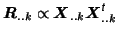
We will therefore estimate the initial temporal Eigenbasis from
for all data sets .
We will therefore estimate the initial temporal Eigenbasis from
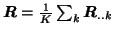 , i.e. by the mean data covariance
matrix. This corresponds to a PPCA analysis of
, i.e. by the mean data covariance
matrix. This corresponds to a PPCA analysis of
 , i.e. the original data reshaped into a
 matrix.
We use the Laplace approximation to the model order [Minka, 2000] to infer on the number of source
processes,
matrix.
We use the Laplace approximation to the model order [Minka, 2000] to infer on the number of source
processes,  . The projection of the data sets onto the matrix
 (formed by
the first common Eigenvectors of
(formed by
the first common Eigenvectors of
 ) reduces the dimensionality of the
data in the temporal domain in order to avoid overfitting. This projection is identical for all
) reduces the dimensionality of the
data in the temporal domain in order to avoid overfitting. This projection is identical for all  different data
sets, given that
is estimated from the mean sample covariance
matrix
. Therefore, we can recover the original time-courses by projection
onto
: when the original
data
different data
sets, given that
is estimated from the mean sample covariance
matrix
. Therefore, we can recover the original time-courses by projection
onto
: when the original
data
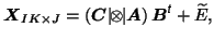
 is transformed into a new set of data
 by projecting each
 onto
, the original data can be recovered from
onto
, the original data can be recovered from
where
 denotes the identity matrix of rank .
If the new data
denotes the identity matrix of rank .
If the new data
 is decomposed such that
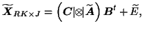 then
then
 where
where
 . This approach is different from
e.g. [Calhoun et al., 2001], where an individual data set is projected onto a
set of Eigenvectors of the data covariance matrix
. This approach is different from
e.g. [Calhoun et al., 2001], where an individual data set is projected onto a
set of Eigenvectors of the data covariance matrix
 . As a
consequence, each data set in [Calhoun et al., 2001] has a different
signal+noise subspace compared to the other data sets.
. As a
consequence, each data set in [Calhoun et al., 2001] has a different
signal+noise subspace compared to the other data sets.
Similar to the 2-D PICA model, the set of pre-processing
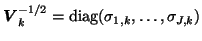
steps is iterated in order to obtain estimates for the
voxel-wise noise variance
 , the PPCA Eigenbasis
 and the
model order before decomposing the reduced data
into the factor matrices
and the
model order before decomposing the reduced data
into the factor matrices
 and
and
 (see [Beckmann and Smith, 2004] for details).
Next: Group-level inference
Up: Tensor PICA
Previous: Relation to mixed-effects GLMs
Christian Beckmann
2004-12-14