Results

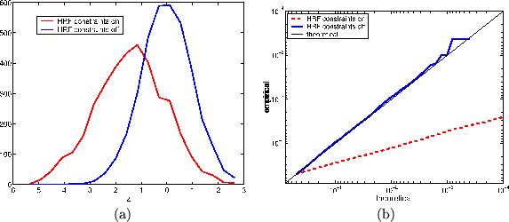
Figure 5(a) shows the histogram of pseudo-z-statistics obtained for the two different models with and without HRF constraints using the Variational Bayesian inference. Figure 5(b) shows the log probability-log probability plots. These show plots of (nominal/theoretical) frequentist FPR against that obtained empirically. The nominal/theoretical FPR is only applicable to the unconstrained HRF model, as we then have noninformative priors and we would expect the Bayesian inference to be equivalent to frequentist inference. Accordingly, the log probability-log probability plot shows good correspondence between the empirically obtained probabilities under the tail for a given z-statistic, and that which we expect from frequentist theory, for the unconstrained HRF model. Recall that to make the inference tractable under Variational Bayes, we introduced a utility parameter, $\phi_{\bar{\beta}_{ie}}$, which we update with point estimates an approximation which may have effected the marginal posterior over $\beta_{ie}$. The fact that we obtain good correspondence here between our inference and the (for this model, known to be correct) frequentist results provides some validation that the marginal posterior over $\beta_e$ is not significantly affected. Unlike the unconstrained model, we would not expect the constrained HRF model to give pseudo-z-statistics that conform to frequentist theory. This is because we now have informative HRF shape priors causing Bayesian inference to be different to frequentist inference. The log probability-log probability plot shows that we get probabilities under the tail for a given z-statistic much smaller empirically than if the frequentist GLM solution held true. The histogram in figure 5(a) shows that this is due to a large shift in the histogram to lower pseudo-z-statistics (the mode is at about $z=-1$). The HRF constraints reduce the power in those voxels where the linear combinations of the basis functions do not give sensible HRF shapes; this produces a shift in the null-distribution histogram. When we have activating voxels with HRF shapes which are not penalised by the HRF prior constraints then the pseudo-z-statistics will not be reduced. We therefore have extra sensitivity when we use Bayesian inference with informative priors constraining the HRF shape.

Figure 5: (a) Histogram of pseudo-z-statistics obtained for the two different models with and without HRF constraints. Figure 5(b) Log probability-log probability plots. These show plots of (nominal/theoretical) frequentist FPR against that obtained empirically. The HRF constraints reduce the power in those voxels where the linear combinations of the basis functions do not give sensible HRF shapes; this produces a shift in the null-distribution histogram.