Shape-specific Intensity Distributions

The above model may be easily extended to include some non-deterministic intensity characteristics for the shapes. For instance, typical shapes are characterised not only by a mean intensity and a spatially-linear intensity gradient, but also by a distribution of intensities about this deterministic intensity model. This distribution can be characterised empirically and used in the similarity model, as done in [,]. Alternatively, the distribution can be approximated by a Gaussian and these variance properties inserted into the above model.

Consider that each shape ($S_j$) is associated with a Gaussian noise process (of length $N$), $\eta_j$, where $\ensuremath{\mathrm{Cov}}(\eta_j) = E(\eta_j \eta_j^{\mathrm{\textsf{T}}}) = \sigma_j^2 I$. The model of image formation is now $Y = G \alpha + \sum_j W_j \eta_j + \epsilon$, where $W_j$ is an $N$ by $N$ weighting matrix given by $\mathrm{diag}(G_1(T(S_j)))$ - i.e. a diagonal matrix where the diagonal elements are taken from the vector $G_1(T(S_j))$. This weighting is such that the noise process $\eta_j$ will only affect voxels that overlap $S_j$ and will not affect other voxels.

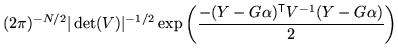
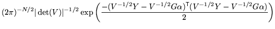
The random component of this model is $\sum_j W_j \eta_j + \epsilon = Y - G \alpha$ and is a multivariate Gaussian with covariance of $\ensuremath{\mathrm{Cov}}(Y - G \alpha) = \sum_j \sigma_j^2 W_j W_j^{\mathrm{\textsf{T}}}+ \sigma^2 I = V$. As a consequence the likelihood becomes

$$p(Y\vert T,S,\theta) = (2 \pi)^{-N/2} \vert \det(V) \vert^{-1/2} \exp\left( \frac{- (Y - G\alpha)^{\mathrm{\textsf{T}}}V^{-1} (Y - G \alpha)}{2} \right)$$

$$= (2 \pi)^{-N/2} \vert \det(V) \vert^{-1/2} \exp\left( \frac{- (V^{... ...1/2} G\alpha)^{\mathrm{\textsf{T}}}(V^{-1/2} Y - V^{-1/2} G \alpha)}{2} \right)$$

which is the same form as before, but with $\beta = 1$, $Y$ replaced by $V^{-1/2} Y$ $G$ replaced by $V^{-1/2} G$ and the prefactor $\vert \det(V) \vert^{-1/2}$ inserted. Therefore all previous results hold with these substitutions. Note that this is only true when $V$ has a nearly block diagonal structure (with few cross-terms between shapes) which is the case for this modelling with non-overlapping shapes.

The posterior for this new model now also depends upon the parameters, $\sigma_j$ (or $\beta_j = \sigma_j^{-2}$) which can be either treated as known parameters, or marginalised numerically. Their effect on the projection matrices and determinants is such that analytical marginalisation is intractable. Also, it is often more convenient to subsume the measurement noise, $\epsilon$, with the new random processes, $\eta_j$, in order to simplify the model and marginalisation. This simply has the effect of changing the values of $\sigma_j$ that will be used (or integrated over) in practice, since all of these processes are considered independent.