Example Box: Spatial Transformations
Introduction
The aim of this example is to become familiar with different types of spatial transformations - both how to apply and view them and the results.
This example is based on tools available in FSL, and the file names and instructions are specific to FSL. However, similar analyses can be performed using other neuroimaging software packages.
Please download the dataset for this example here:
Data download
The dataset you downloaded contains the following:
- Original (non-brain-extracted) structural image:
S01.nii.gz - A brain extracted image:
S01_brain.nii.gz - Linear spatial transformations (matrices):
S01_lin_6dof.matandS01_lin_12dof.mat - Nonlinear spatial transformation (warp):
S01_warp.nii.gzandS01_coef.nii.gz - Image results of the above transformations:
S01_lin_brain_6dof.nii.gz, S01_lin_brain_12dof.nii.gzandS01_nonlin.nii.gz
S02). Both of these subjects are from the same dataset used to generate Figure 5.9 in the Primer.
Viewing the Data
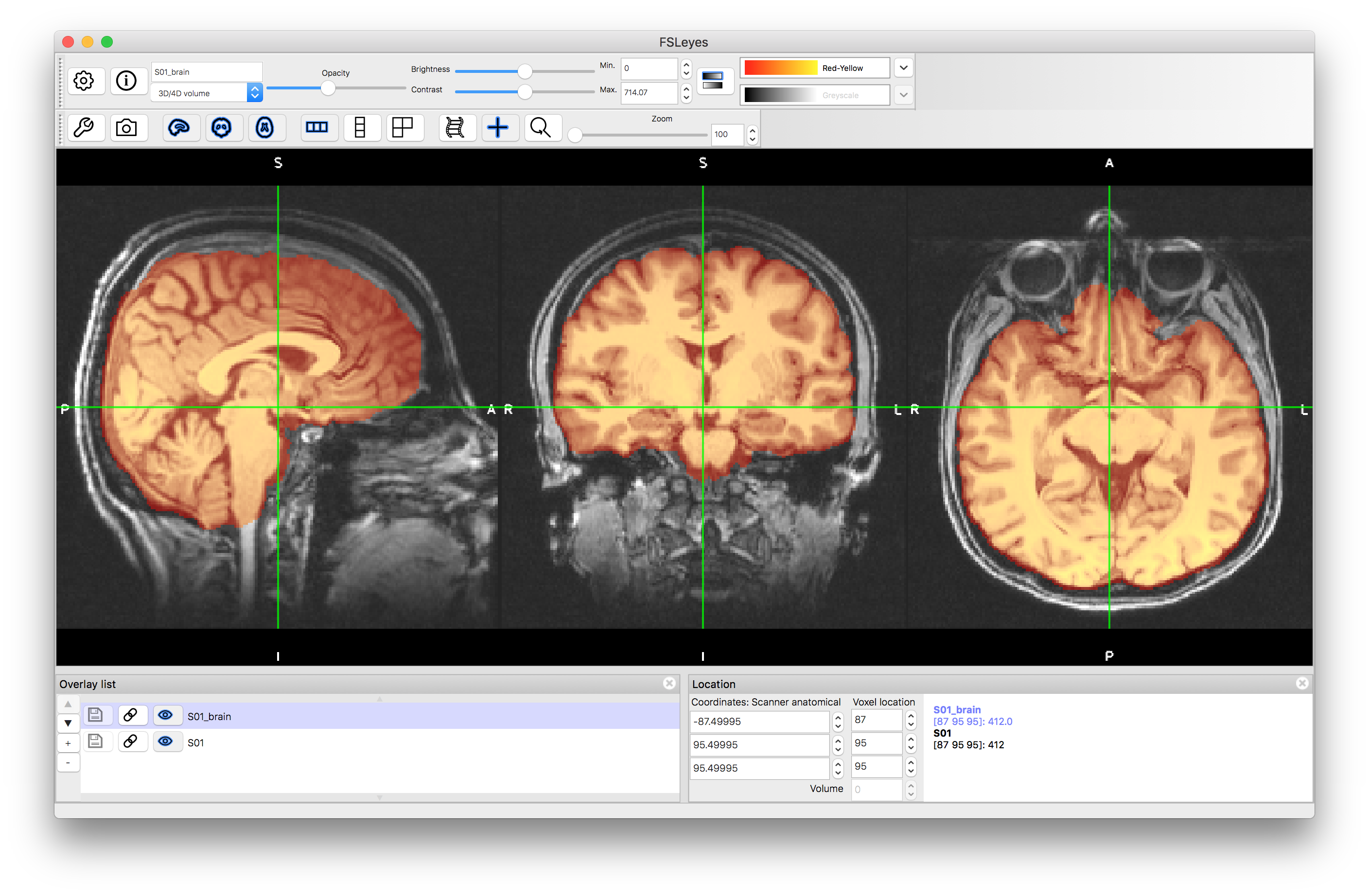
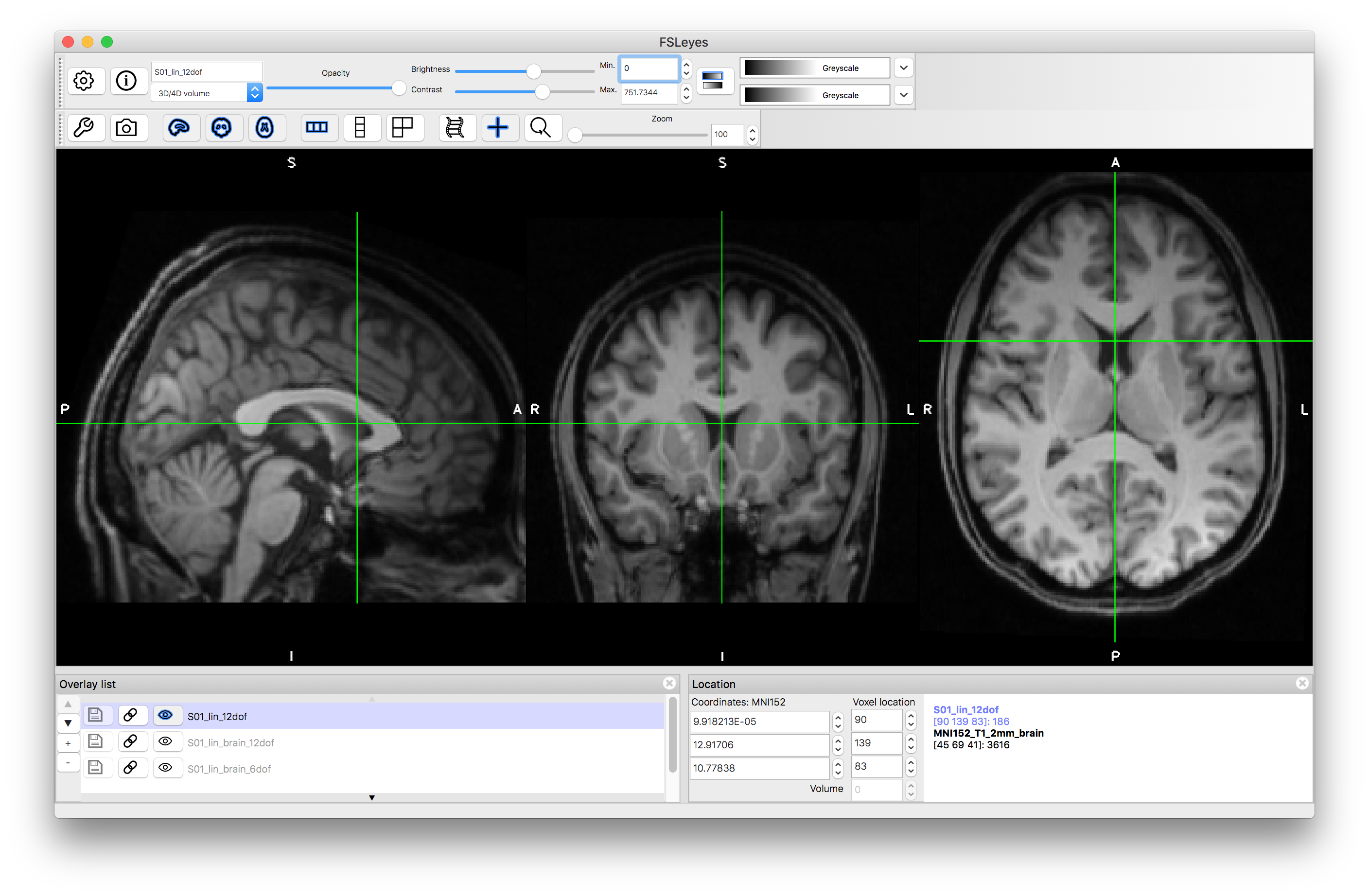
To start with load the original image (S01.nii.gz) into a viewer (e.g. fsleyes) and inspect it. Then load the brain extracted image (S01_brain.nii.gz) and view it. Note that although the extraction is not perfect it is sufficiently good for registration purposes.
Linear Registrations
Spatial Transformations
We will consider the registration of this subject to the standard MNI152 template. In this case the FSL tool for linear registration, FLIRT, has been used to create to registrations, each based on the brain extracted images: S01_brain and MNI152_T1_2mm_brain. Using brain extracted images for this stage is the recommended approach in FSL, to avoid non-brain features driving the registration.
Two versions of the registrations have been run: one with 6 DOF (rigid-body) and one with 12 DOF (affine). Click here to see the command line used (though note that you do not need to run this or understand it at this point).
The resulting spatial transformations from these are saved in the files S01_lin_6dof.mat and S01_lin_12dof.mat and store 4 by 4 matrices that encode all the relevant information. These can be viewed by running (in a terminal) the command:
cat S01_lin_6dof.mat
and similarly for the 12 DOF version. You should see the matrices displayed as below:
0.9994542042  0.02747834671  0.01833678658  -3.421860238
-0.0319232723  0.9461499184  0.3221508976  -2.555450438
-0.008497175771  -0.3225604645  0.9465106349  9.763313161
0  0  0  1
12 DOF:
1.053957719  0.02720367834  0.01853985618  -8.327319065
-0.03122847873  1.168361562  0.3943113963  -28.37072248
0.0006216970311  -0.3947374238  1.179723167  -15.37194263
0  0  0  1
It is not easy to gain much useful information by looking at these matrices directly. In fact, it is not even straightforward to tell the difference between a 6 DOF and a 12 DOF transformation (as each typically have 12 non-zero values). It is more informative to look at the decomposition of these matrices in terms of parameters. This can be done in FSL using the command:
avscale --allparams S01_lin_6dof.mat
which gives quite a lot of output, including the following lines:
Rotation Angles (x,y,z) [rads] = 0.328058 -0.018338 0.027486
Translations (x,y,z) [mm] = -3.421860 -2.555450 9.763313
Scales (x,y,z) = 1.000000 1.000000 1.000000
Skews (xy,xz,yz) = 0.000000 0.000000 0.000000
and similarly for the 12 DOF case, although with more interesting scales and skews (since for 6 DOF they are fixed to scalings of 1.0 and skews of 0.0, as shown above).
Image Outputs
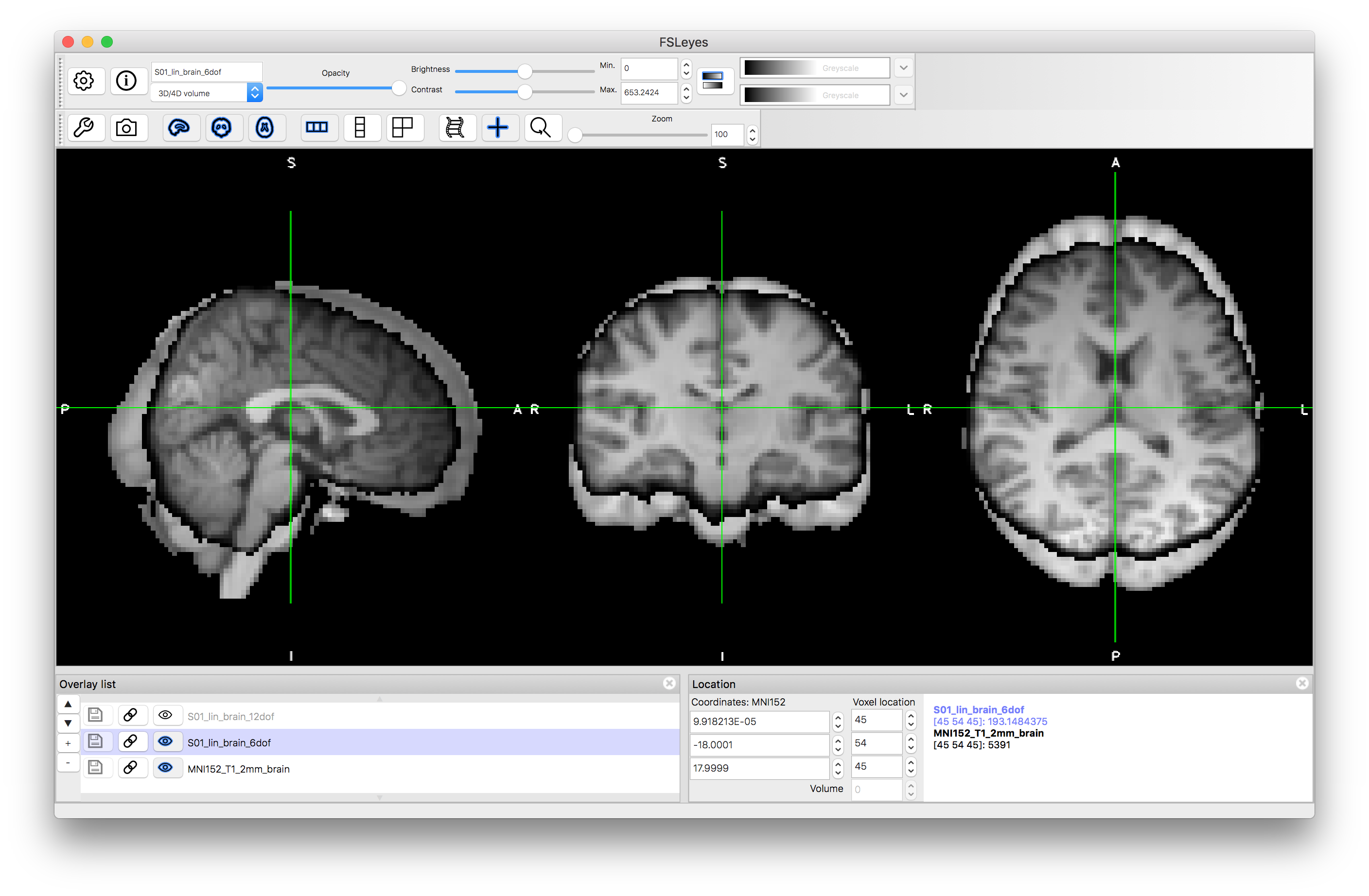
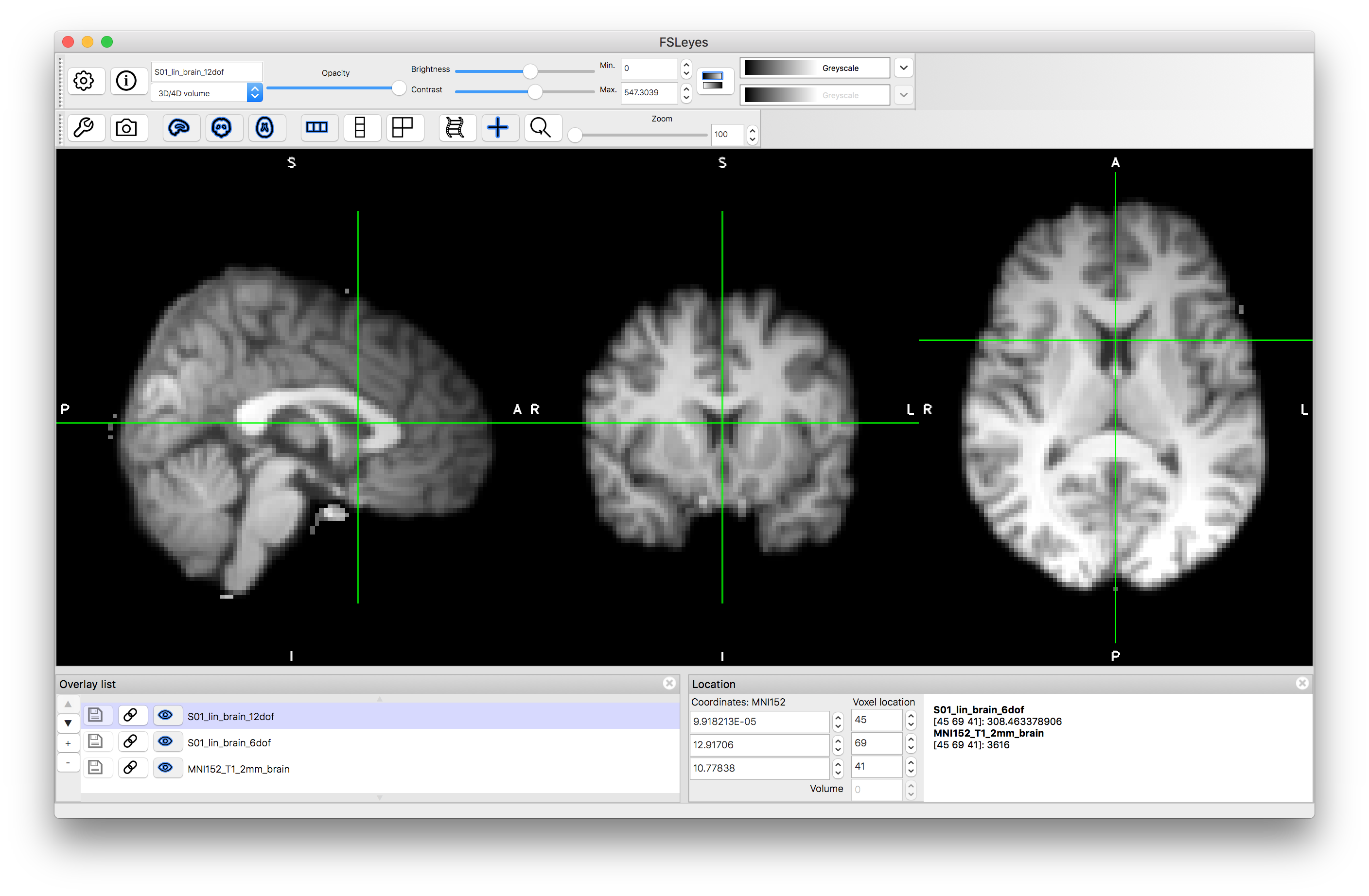
Now view the images that correspond to the outputs of these registrations. To do this you want to compare to the reference image, so close the previous views or start a new viewer, and load the standard image: MNI152_T1_2mm_brain (use File -> Add standard in fsleyes). Add the images S01_lin_brain_6dof.nii.gz and S01_lin_brain_12dof.nii.gz on top of this. Try flicking between the images (e.g. turning the visibility on and off using the "eye" icon in the Overlay list) or using a side-by-side view (e.g. adding an extra "ortho view" from the View menu) to investigate how well aligned the images are. It should be obvious that the 6 DOF alignment gets the approximate rotation and orientation correct but the brain has a very different size to the MNI152 template brain. The 12 DOF result is much better in terms of overall size, but still has noticeable inaccuracies.
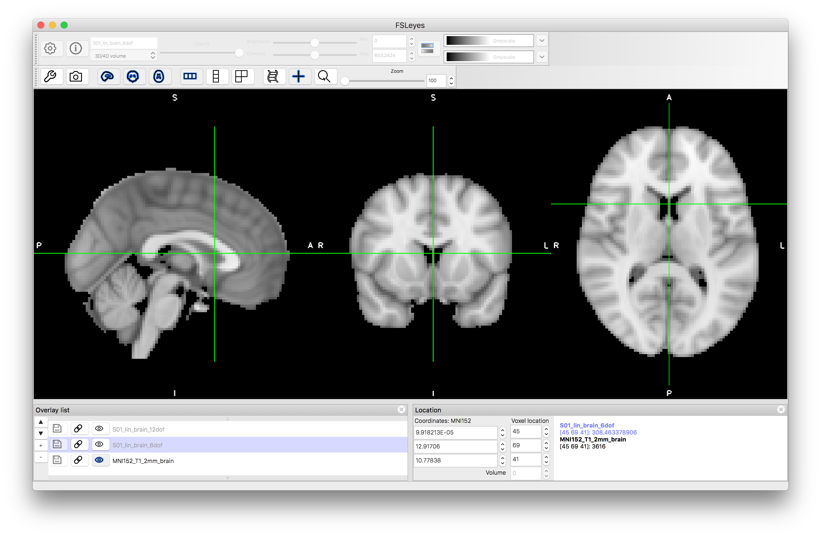
6 DOF result:
12 DOF result:
Applying Transformations
Another thing that you might have noticed when viewing the images was that the resolution was low (2mm), as this reflected what was used as the reference image in the registration command. Using this lower resolution is sufficient for running registrations to obtain the spatial transformations. It is also possible to apply the spatial transformation to the original image to obtain a higher resolution result. The following command will create an image with 1mm resolution, and using the whole image, not just the brain-extracted version:
flirt -in S01.nii.gz -ref $FSLDIR/data/standard/MNI152_T1_1mm -applyxfm -init S01_lin_12dof.mat -out S01_lin_12dof.nii.gz
After running the above command, load the resulting image S01_lin_12dof.nii.gz and note that the resolution is 1mm (determined by the reference image resolution in the above command) whilst the alignment of the brain is precisely the same. Also note that this output contains all the non-brain structures as well. If you wanted to have a high resolution version of the brain-extracted image instead then repeat the above command but replace S01.nii.gz with S01_brain.nii.gz.
Nonlinear Registrations
Spatial Transformations
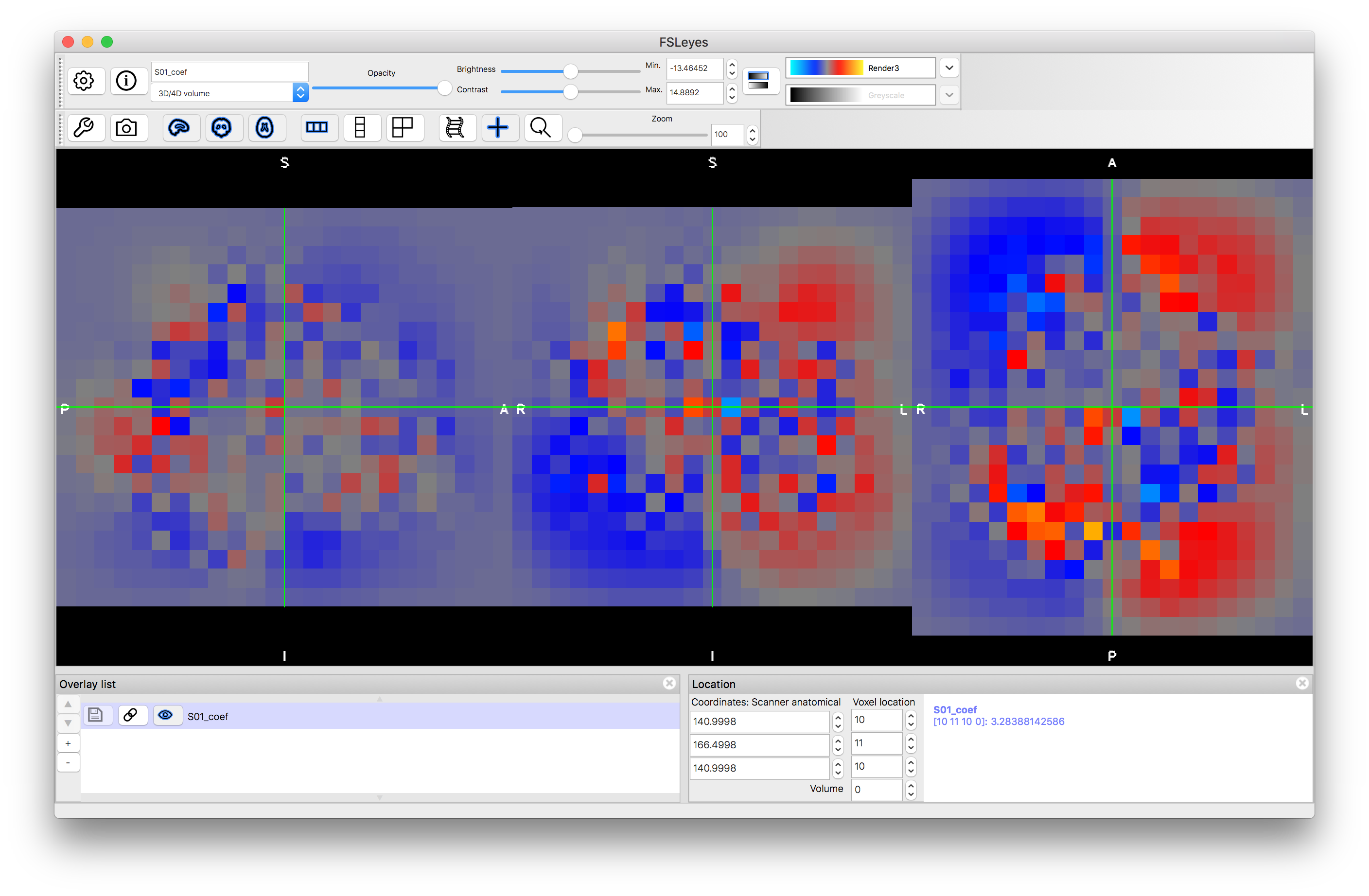
Start a new viewer and load the image S01_coef.nii.gz, then change the colourmap to "Render3". This image represents the nonlinear spatial transformation in the native format for FSL (a coefficient file), which is similar to a low resolution representation of a warp field. This is a 4D volume, consisting of three 3D volumes: change the "Volume" number from 0 to 1 and then 2, to see these. Each volume represents a component of the warp (or displacement) vectors: 0 = x component, 1 = y component and 2 = z component.
The image S01_warp.nii.gz contains a higher resolution version of the warp field in a format that is more directly interpretable (the intensity values, put together across the 3D volumes, form the displacement vector in units of mm). Load this image and place the cursor at the voxel location (27, 41, 69). Look at the intensity values at this location in the different volumes, which should be: 6.85, -36.98, 11.25. This represents the amount that this voxel has been moved by the transformation (i.e. 6.85 mm in x, -36.98 mm in y and 11.25 mm in z). It is this information that completely defines the transformation. Either of these files (the warp or the coef) can be used to apply this transformation to other images.
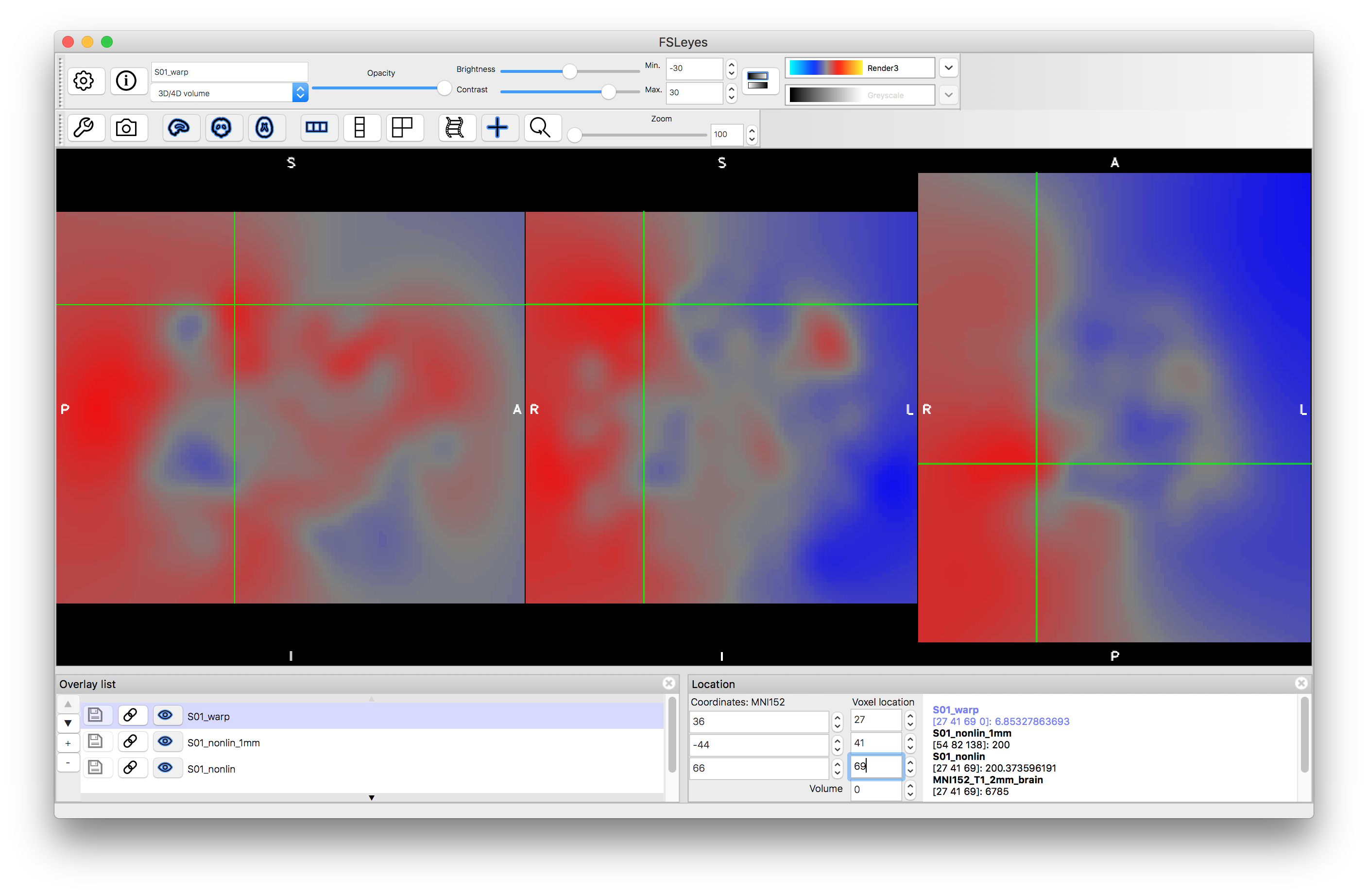
Image Outputs
Load the output image S01_nonlin.nii.gz on top of the MNI152_T1_2mm standard image. Inspect the images and verify how much better the alignment is by comparison with the previous linear registrations. Note that linear registrations are still essential for initialisation of the nonlinear registration, and rigid-body registrations are the appropriate, and accurate, registrations to use for within-subject registrations.

Applying Transformations
To make a higher resolution version of the output, you can apply the transformation with the following command:
applywarp -i S01.nii.gz -r $FSLDIR/data/standard/MNI152_T1_1mm -w S01_warp.nii.gz -o S01_nonlin_1mm.nii.gz
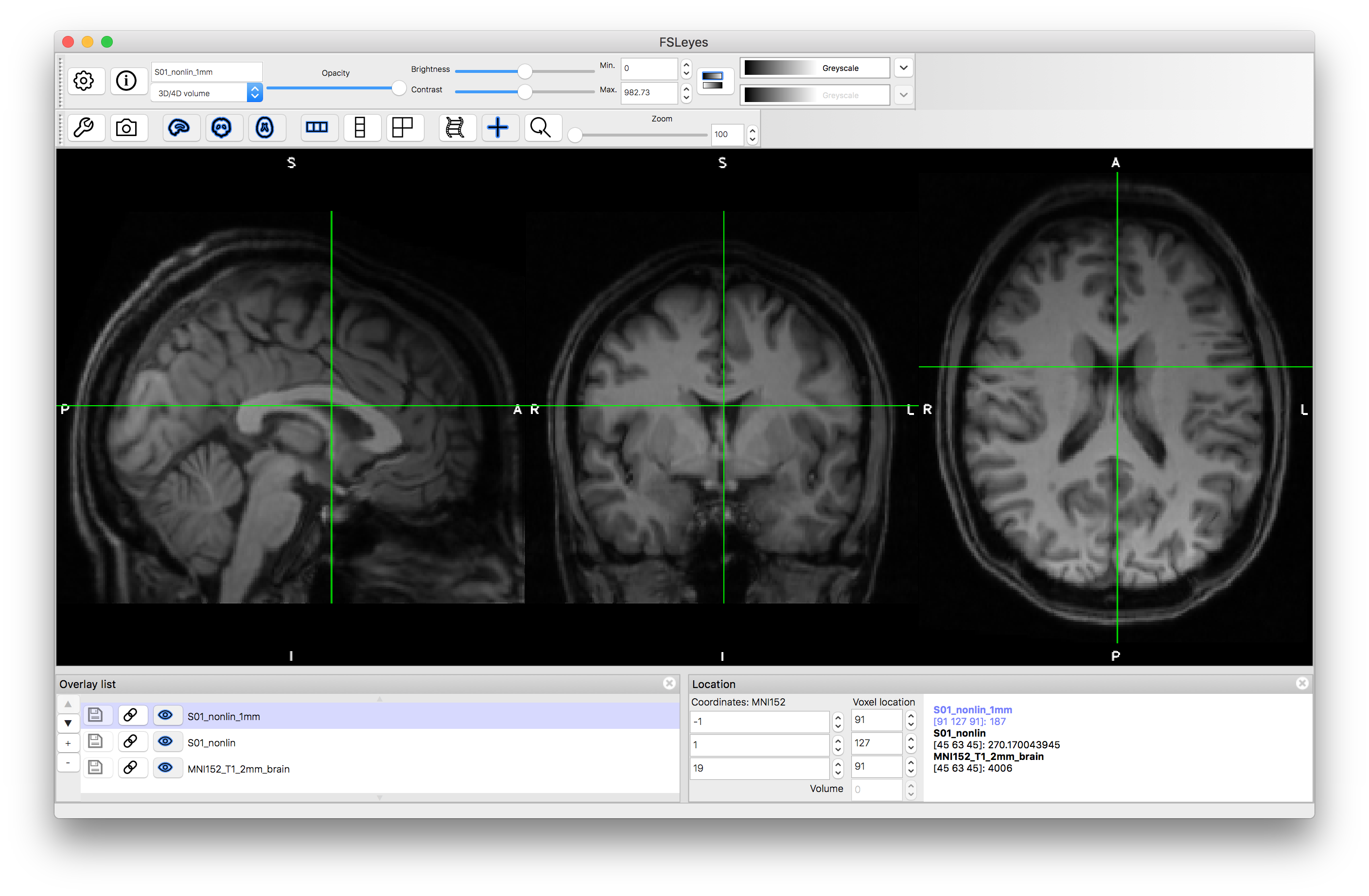
A similar command can be run to transform other images from the structural space to the MNI standard space (e.g. segmentations, such as would be produced in a VBM pipeline). Both the linear and nonlinear versions of applying transformations use the same principles - with a Field of View (FOV) and resolution determined by the reference image (the content of the reference is not used, only the FOV and resolution), in order to transform the input image according to the spatial transformation (matrix or warp). Applying transformations like this is commonly done in many points within analysis pipelines, and requires that the transformation files are saved.
From these examples you should have an understanding of what format the spatial transformations are saved as, and how to apply these transformations to images. In addition, it demonstrates what alignments look like with the different transformations in this example (of registering a structural image to the MNI standard space). Try repeating the above steps with the other subject (S02) to see how this works in a different image, as this second subject is older and has noticeably larger ventricles.