Example Box: Tissue-Type Segmentation

Introduction

The aim of this example is to become familiar with running tissue-type segmentation and interpreting the outputs.

This example is based on tools available in FSL, and the file names and instructions are specific to FSL. However, similar analyses can be performed using other neuroimaging software packages.

Please download the dataset for this example here:

Data download

The dataset you downloaded contains the following files:

Structural image: structural.nii.gz
Brain extracted image: structural_brain.nii.gz
Segmented images: structural_brain_pve_0.nii.gz, structural_brain_pve_1.nii.gz and structural_brain_pve_2.nii.gz
Bias-corrected image: structural_brain_restore.nii.gz
Second structural image (brain extracted): T1_brain.nii.gz
Bias-corrected version: T1_brain_restore.nii.gz

Viewing the Data

Load the original structural image into a viewer (e.g. fsleyes) and the add the segmented images. For each for the segmented images set the display range (min/max) to 0.5 to 1.0. Also set a different color scheme for each of these segmented images (e.g., red for PVE 0, green for PVE 1, blue for PVE 2).

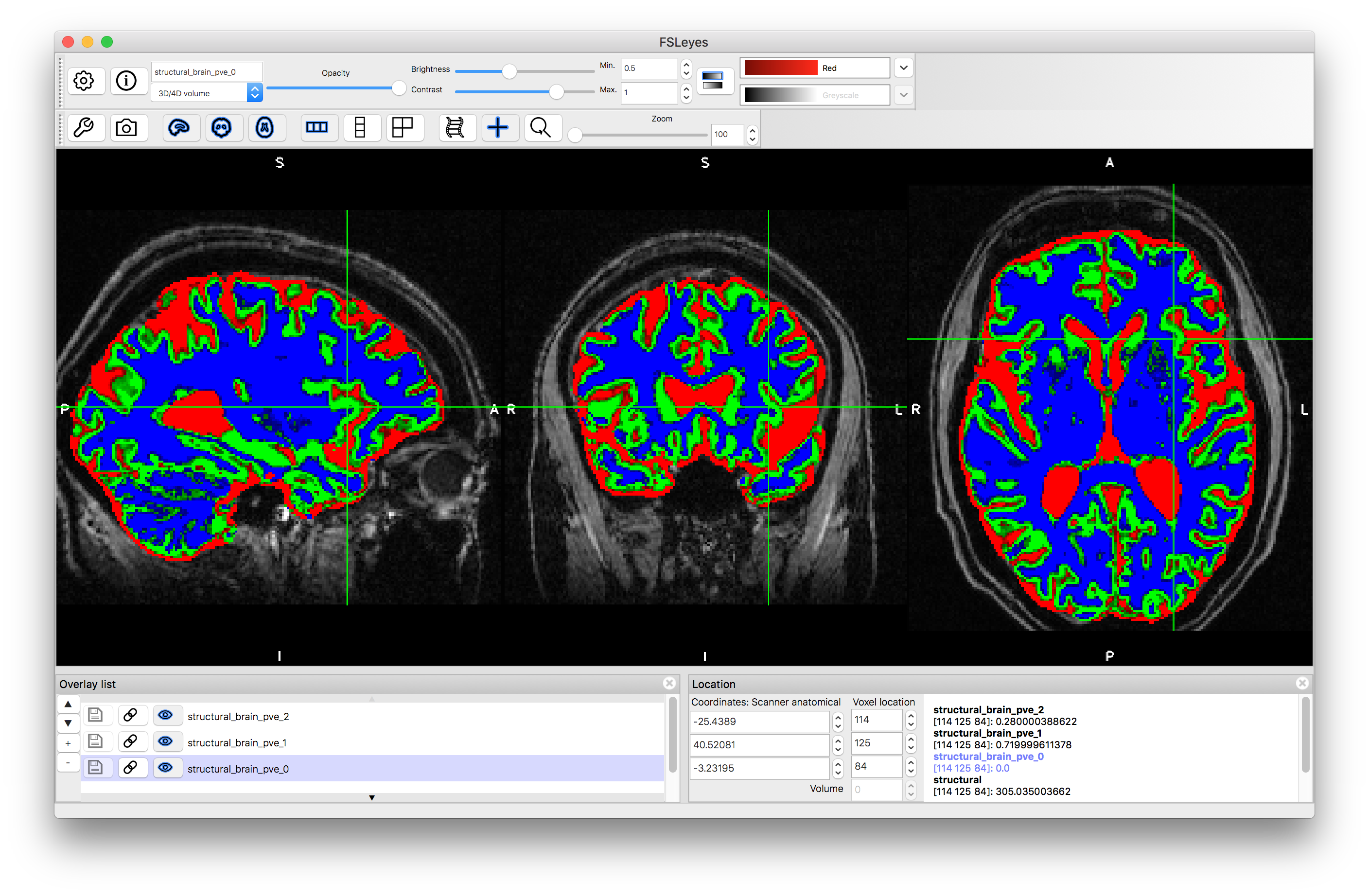
Each PVE image represents the Partial Volume Estimate for a particular tissue. The numbering is determined by the average intensity of each tissue, ordered from darkest to brightest, which in the case of a T1-weighted image (as we have here) gives: PVE 0 = CSF ; PVE 1 = Gray Matter ; PVE 2 = White Matter. At each voxel the number stored in this image (the "intensity" that is displayed in the bottom right part of fsleyes).

If you choose a location at the edge of the cortex (as shown in the above image) you will see that the partial volume is zero for one tissue but substantially different for the other two. For example, at voxel location (114, 125, 84) the values are 0.0, 0.72 and 0.28 for the three tissues respectively. This represents the fact that at this voxel there is a mixture of gray matter and white matter, with the estimate being 72% gray matter and 28% white matter.

Try selecting other locations and seeing what the values of the partial volumes are. In particular, look at some of the deep gray matter structures, such as the thalamus or putamen, which have substantial mixtures of gray matter and white matter, reflecting the biology where there can be significant amounts of axons within these structures.

Running Segmentation

The above segmentation can be easily run with FSL using the following command in a terminal (see general instructions on how to run FSL commands here):

fast -B structural_brain

The -B option is used to make it output the bias-corrected image (see below), as well as the PVE images above, and some other summaries (such as the pveseg image where each voxel is labelled according to the tissue that has the maximum PVE). Other outputs are also possible - see the FSL wiki for more information.

Bias-Field Correction

In the first image above there is very little bias field (uneven intensities due to RF, or B₁, inhomogeneities), so that the bias-corrected image structural_brain_restore.nii.gz is almost identical to the original image. However, the second image T1_brain.nii.gz contains a very strong bias field and so the bias-corrected output T1_brain_restore.nii.gz. This can be easily seen by viewing the two images and "flicking" between them (i.e., clicking the top one on and off in the image list using the "eye" icon, or by moving the opacity slider). This shows how such bias fields can be corrected, although note that the noise then becomes very uneven, with noticeably higher noise in the posterior parts of the brain, wherever the original intensities were lower.

These examples should help to demonstrate what tissue-type segmentation is capable of and how to interpret the outputs. Remember that brain extraction, which has been done for you in these examples, is a necessary first step, prior to segmentation.