Results

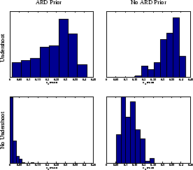
Figures 5(a) and 6(a) show the fit at a typical voxel in the dataset generated with and without undershoot respectively. Figures 5(b) and 6(b) show 11 evenly spread samples from the posterior of the HRF for the same voxel. For the four combinations of two datasets (generated with and without undershoot) and different models (with and without ARD prior on the undershoot) we computed the histograms of the mean of the marginal posterior for undershoot size, $c_2$. We would expect the model fitted without the ARD prior to always fit a post-stimulus undershoot even for the dataset generated without the post-stimulus undershoot. However, the model with the ARD prior should force the undershoot size parameter to close to zero when using the dataset generated without the undershoot, but does fit an undershoot when using the dataset generated with an undershoot. This is exactly what can be seen in figure 7.

Figure 5: Posterior HRF for artificial activation with undershoot. (a) Mean posterior fit (high-pass filtered data as a broken line, response fit as a solid line). (b) 11 evenly spread samples from the posterior of the HRF. The posterior mean HRF is plotted along with different HRFs each of which have one parameter varying at the $\pm 85^{th}$ percentile of the posterior, with the other parameters held at the mean posterior values.

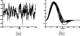Figure 6: Posterior HRF for artificial activation without undershoot. (a) Mean posterior fit (high-pass filtered data as a broken line, response fit as a solid line). (b) 11 evenly spread samples from the posterior of the HRF. The posterior mean HRF is plotted along with different HRFs each of which have one parameter varying at the $\pm 85^{th}$ percentile of the posterior, with the other parameters held at the mean posterior values.

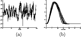Figure 7: Histograms of the posterior mean of the HRF characteristic, $c_2$, corresponding to the relative size of the post-stimulus undershoot. [top] Artificial dataset generated with undershoot ( $c_{i2}=0.3$). [bottom] Artificial dataset generated without undershoot. [left] ARD prior. [right] no ARD prior. This illustrates how the ARD prior forces the undershoot to be zero when there is insufficient evidence to support it in the data. Without the ARD prior a non-zero undershoot is inferred when no undershoot actually exists. The ARD prior protects against overfitting.