


Next: Space-Time Simultaneously specified Auto-Regressive
Up: Small Scale Variation
Previous: Small Scale Variation
One approach to simplifying equation 3 is to consider a stationary
separable model (28,1). This gives:
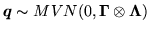 |
(4) |
where  represents the Kronecker product and where
 and
and
 are the spatial (
 ) and temporal
(
) and temporal
( ) covariance matrices respectively. This is where the
covariance between two observations is decomposed into the
temporal covariance at the lag between the observations multiplied
by the spatial covariance at the distance between the
observations. Such a decomposition would make computation a lot
easier, for example when computing the inverse, which is necessary
for all viable inference techniques. The use of equation
4 means that the spatial autocovariance is
assumed to be the same at all time points. This seems a reasonable
assumption. However, it also requires that the temporal
autocovariance is the same at all voxels. Previous
studies (43,13), clearly demonstrated that
this was not the case and would be an incorrect assumption to
make. Consequently, a separable model is not considered further.
) covariance matrices respectively. This is where the
covariance between two observations is decomposed into the
temporal covariance at the lag between the observations multiplied
by the spatial covariance at the distance between the
observations. Such a decomposition would make computation a lot
easier, for example when computing the inverse, which is necessary
for all viable inference techniques. The use of equation
4 means that the spatial autocovariance is
assumed to be the same at all time points. This seems a reasonable
assumption. However, it also requires that the temporal
autocovariance is the same at all voxels. Previous
studies (43,13), clearly demonstrated that
this was not the case and would be an incorrect assumption to
make. Consequently, a separable model is not considered further.
Next: Space-Time Simultaneously specified Auto-Regressive
Up: Small Scale Variation
Previous: Small Scale Variation