Results

Figures 3--7 show the results of inferring on the three different continuous weights mixture models on the five different artificial datasets. The spatial maps in the figures are unthresholded marginal posterior means of $w_{ik}$, i.e. $E_{w_{ik}\vert y}(w_{ik})$, for all three classes of deactivation, non-activation and activation.

We can compute the effective global class proportions based upon the classifications, i.e.:

$${\tilde{\pi}}_k=\frac{\sum_{i\in k} \bar{w}_{ik}}{\sum_{ik} \bar{w}_{ik}}$$ (25)

where the weights $\bar{w}_{ik}$ are the mean marginal posterior weights. These effective global class proportions can be combined with the mean marginal posterior class distribution parameters to give a histogram fit. These are shown in figures 3--7(a).

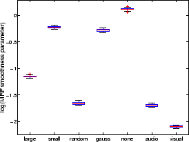
The box plot in figure 8 shows the marginal posterior distributions of the MRF smoothness parameter $\phi_{\tilde{w}}$ for the different artificial datasets. The value of $\phi_{\tilde{w}}$ clearly varies a lot from dataset to dataset emphasising the need for adaptive determination of the spatial smoothness.

It is interesting to compare model 2's performance with that of model 3. Model 3 is the same as model 2, except that in model 3 the spatial regularisation parameter is adaptive and in model 2 it is fixed. Model 2 works well on some datasets, for example figures 6 and 7. This is because the arbitrarily chosen value of $\phi_{\tilde{w}}=1$ is close to the adaptively determined values of $\phi_{\tilde{w}}$ for those datasets, which can be seen in figure 8 (note that $log(1)=0$). 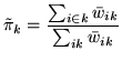For the other datasets it works less well. For example, it overblurs the edges in figure 3 and overblurs the activation and deactivation to the point of removing much of it in figures 4 and 5.

It is worth emphasising that model 3 also works well on the no activation dataset (figure 7). This is a dataset where there is in fact only one class present (the non-activation class), and yet we fit the mixture model assuming three classes. Despite this, model 3 forces all probabilities to well less than $0.5$ for the activation and deactivation classes.

Figure 3: Results for the large activation artificial dataset. Top left is the actual data, $y_i$. (a) shows the histograms of $y_i$ along with the fit for the different mixture models (the red lines show the individual class distributions and the dashed yellow line shows the overall fit). (b) Spatial maps of unthresholded $w_{ik}$ for [left] deactivation [middle] non-activation [right] activation.

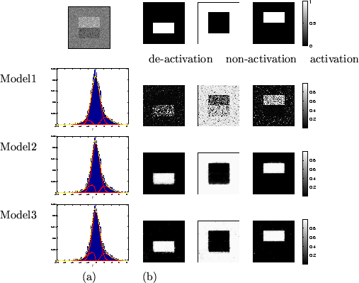Figure 4: Results for the small activation artificial dataset. Top left is the actual data, $y_i$. (a) shows the histograms of $y_i$ along with the fit for the different mixture models (the red lines show the individual class distributions and the dashed yellow line shows the overall fit). (b) Spatial maps of unthresholded $w_{ik}$ for [left] deactivation [middle] non-activation [right] activation.

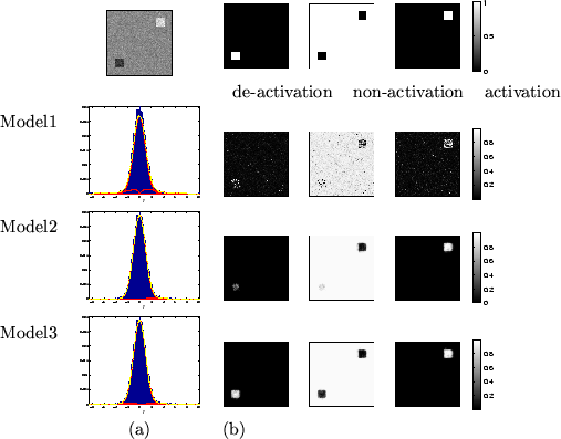Figure 5: Results for the random checker activation artificial dataset. Top left is the actual data, $y_i$. (a) shows the histograms of $y_i$ along with the fit for the different mixture models (the red lines show the individual class distributions and the dashed yellow line shows the overall fit). (b) Spatial maps of unthresholded $w_{ik}$ for [left] deactivation [middle] non-activation [right] activation.

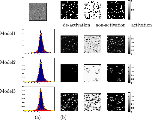Figure 6: Results for the Gaussian activation artificial dataset. Top left is the actual data, $y_i$. (a) shows the histograms of $y_i$ along with the fit for the different mixture models (the red lines show the individual class distributions and the dashed yellow line shows the overall fit). (b) Spatial maps of unthresholded $w_{ik}$ for [left] deactivation [middle] non-activation [right] activation.

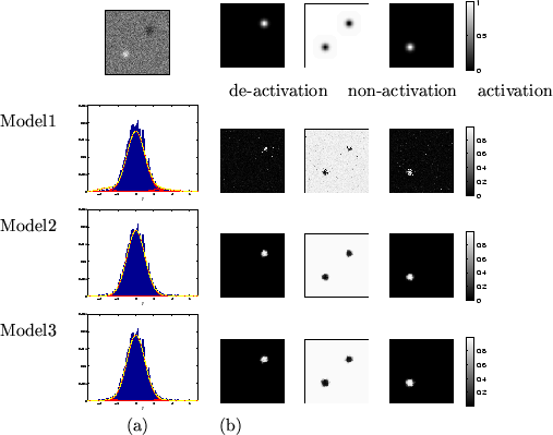Figure 7: Results for the no activation artificial dataset. Top left is the actual data, $y_i$. (a) shows the histograms of $y_i$ along with the fit for the different mixture models (the red lines show the individual class distributions and the dashed yellow line shows the overall fit). (b) Spatial maps of unthresholded $w_{ik}$ for [left] deactivation [middle] non-activation [right] activation.

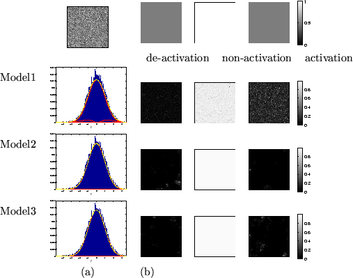Figure: Box plot showing the marginal posterior distributions of the MRF smoothness parameter $\phi_{\tilde{w}}$ for the different datasets. The value of $\phi_{\tilde{w}}$ clearly varies a lot from dataset to dataset emphasising the need for adaptive determination of the spatial smoothness.