


Next: Continuous Weights Mixture Model
Up: Discrete Labels Mixture Model
Previous: Non-spatial with Class Proportions
The prior on  is now a spatial prior. In this work we
assume a discrete MRF (Besag, 1986; Geman and Geman, 1984). Taking
is now a spatial prior. In this work we
assume a discrete MRF (Besag, 1986; Geman and Geman, 1984). Taking
 , where
  is the MRF control
parameter, which controls the amount of spatial regularisation. We
have:
is the MRF control
parameter, which controls the amount of spatial regularisation. We
have:
![$\displaystyle p(\vec{x}=\vec{\kappa}\vert\phi_x)\propto f(\phi_x)exp \left(-\frac{\phi_x}{4} \sum_i \sum_{j\in{\cal N}_i} I[x_i \neq x_j] \right)$](img41.png) |
(6) |
where
 is the spatial neighbourhood of
  (for this
we use 26-connectivity in 3-dimensions),
(for this
we use 26-connectivity in 3-dimensions),
![$ I[x_i \neq x_j]$](img43.png) is an
indicator function (it is one if
is an
indicator function (it is one if
 and is zero
otherwise), and
and is zero
otherwise), and  is some unknown function of .
This prior is identical to the prior used
in Zhang et al. (2001); Salli et al. (1999), if the parameter is set to
one. Usually, is hand tuned to work well for particular
types of dataset. The ``best'' value for will depend on
the amount of, and topography of, the different classes.
Marroquin et al. (2003) refer to this as the parameter which controls
the granularity of the field, and they discuss how the use of
different values for this parameter can affect the resulting
segmented field. Indeed, we shall demonstrate later how fixing the
amount of spatial regularisation to a single value will perform
considerably less well than determining it adaptively from the
data.
is some unknown function of .
This prior is identical to the prior used
in Zhang et al. (2001); Salli et al. (1999), if the parameter is set to
one. Usually, is hand tuned to work well for particular
types of dataset. The ``best'' value for will depend on
the amount of, and topography of, the different classes.
Marroquin et al. (2003) refer to this as the parameter which controls
the granularity of the field, and they discuss how the use of
different values for this parameter can affect the resulting
segmented field. Indeed, we shall demonstrate later how fixing the
amount of spatial regularisation to a single value will perform
considerably less well than determining it adaptively from the
data.
The hyperprior we use on is a
non-informative Gamma distribution:
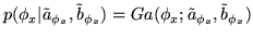 |
(7) |
Using all of this in equation 1,
the posterior becomes:
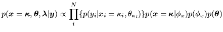 |
(8) |
Clearly, a fourth mixture model could be considered. This would be
a spatial mixture model with global class proportions. However, it
is far from clear how we would combine the prior on  in
equation 4 with that in equation 6.
Anyway, as we shall see in the results, we obtain good global
histogram fits with the spatial mixture model specified here without
including global class proportions.
in
equation 4 with that in equation 6.
Anyway, as we shall see in the results, we obtain good global
histogram fits with the spatial mixture model specified here without
including global class proportions.
Next: Continuous Weights Mixture Model
Up: Discrete Labels Mixture Model
Previous: Non-spatial with Class Proportions