


Next: Discussion
Up: FMRI data
Previous: Methods
Figure 7 shows the posterior means of the AR parameters
from the single-event pain dataset for two different models: with
non-spatial and with spatial MRF AR parameter priors. For the model with
spatial MRF priors, the Variational Bayesian inference adaptively
determines the amount of spatial regularisation to impose for each
of the autoregressive parameter MRFs separately. The spatial maps
for  are very similar, but as we increase
  the MRF spatial
regularisation increases. This shows how the adaptive
determination of the amount of spatial regularisation
automatically adjusts to avoid overfitting of the high order
autoregressive parameters.
In terms of inference on the normalised power of the
f-contrasts, figure 8(a) suggests that
avoiding overfitting and spatially regularising the AR parameters
does make a significant difference to the pseudo-z-statistics.
the MRF spatial
regularisation increases. This shows how the adaptive
determination of the amount of spatial regularisation
automatically adjusts to avoid overfitting of the high order
autoregressive parameters.
In terms of inference on the normalised power of the
f-contrasts, figure 8(a) suggests that
avoiding overfitting and spatially regularising the AR parameters
does make a significant difference to the pseudo-z-statistics.
Figure 7:
Posterior means of parameters from an autoregressive
model of order 4 from the single-event pain dataset.
From left to right we have increasing from  to
to  .
We show this for two different priors on the AR parameters:
[top] non-informative non-spatial, and
[bottom] spatial MRF.
.
We show this for two different priors on the AR parameters:
[top] non-informative non-spatial, and
[bottom] spatial MRF.
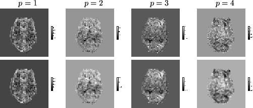 |
Figure 8:
Histogram of the voxelwise
difference in pseudo-z-statistics between
the model with
non-spatial non-informative AR priors and the model with
adaptive spatial MRF AR priors for the single-event pain dataset.
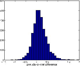 |
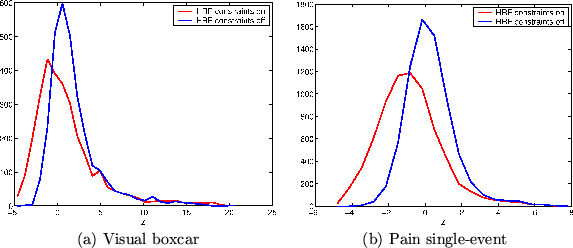
Figure 9 shows the histogram of
pseudo-z-statistics obtained for the two different models with and
without HRF constraints. For both conditions we can see how the
right hand tail, i.e. those voxels which are strongly activating,
is relatively unaffected. Whereas, the main body of the histogram,
i.e. the background non-activating voxels, is shifted to the left
in the same way that it was for the null artificial data.
Figure 9:
Histogram of pseudo-z-statistics obtained for two
different models (with and without HRF
constraints) on (a) the visual boxcar dataset and (b) the pain
single-event dataset.
 |
Figures 10 and 12 show the
results of applying the spatial mixture modelling on the
unconstrained HRF model. Figures 11
and 13 show the results for the constrained HRF
model. Figure 14 shows the difference in voxel
classification between the constrained HRF model and the
unconstrained HRF model. This difference highlights the increased
sensitivity. With the constrained HRF model smaller strength
activating voxels have increased probability of being in the
activation class. This is because the non-activating class
distribution is shifted to lower pseudo-z-statistics when we use
the constrained HRF model.
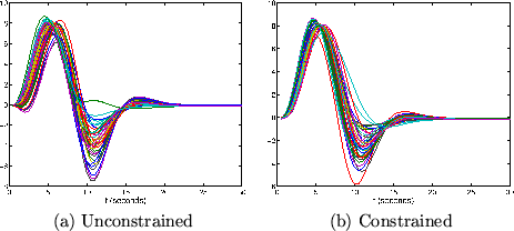
Figures 15 and 16 show samples
from the marginal posterior of the HRF at a voxel which is not
activating and a voxel which is strongly activating respectively
in the pain experiment. In particular, figure 15
highlights the difference between the unconstrained and
constrained HRF models for a non-activating voxel. Whereas, in
figure 16 the HRF shape conforms to prior
expectations, hence there is little different between the
unconstrained and constrained HRF models for a strongly activating
voxel.
Figure 10:
Visual condition. Results of applying the spatial mixture
modelling on the unconstrained HRF model. [top] Pseudo-z-statistic
spatial maps. [bottom] Probability of being in the activation
class. [right] Mixture model fit to histogram of
pseudo-z-statistics.
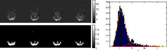 |
Figure 11:
Visual condition. Results of applying the spatial mixture
modelling on the constrained HRF model. [top] Pseudo-z-statistic
spatial maps. [bottom] Probability of being in the activation
class. [right] Mixture model fit to histogram of
pseudo-z-statistics ('A' and 'B' mark the pseudo-z-statistics for
which voxels with greater pseudo-z-statistics have higher
probability of being active than non-active for the constrained
HRF model and unconstrained HRF model
respectively).
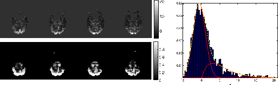 |
Figure 12:
Pain single-event condition. Results of applying the
spatial mixture modelling on the unconstrained HRF model. [top]
Pseudo-z-statistic spatial maps. [bottom] Probability of being in
the activation class. [right] Mixture model fit to histogram of
pseudo-z-statistics.
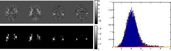 |
Figure 13:
Pain single-event condition. Results of applying the
spatial mixture modelling on the constrained HRF model. [top]
Pseudo-z-statistic spatial maps. [bottom] Probability of being in
the activation class. [right] Mixture model fit to histogram of
pseudo-z-statistics ('A' and 'B' mark the pseudo-z-statistics for
which voxels with greater pseudo-z-statistics have higher
probability of being active than non-active for the constrained
HRF model and unconstrained HRF model
respectively).
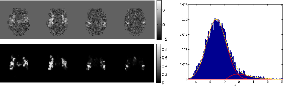 |
Figure 14:
Difference in voxel classification between the
constrained HRF model and the unconstrained HRF model. [red]
voxels are active for both models, [blue] voxels are active for
just the unconstrained HRF model, and [yellow] voxels are active for
just the constrained HRF model. Voxels are classified as
activating with probability of being in the activation class
greater then 0.5. [top] Visual boxcar dataset [Bottom] Pain
single-event dataset.
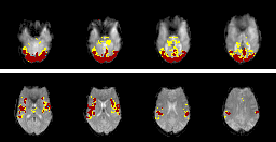 |
Figure 15:
Samples from the marginal posterior of the HRF at a
single voxel which is not activating in the pain experiment. (a)
Unconstrained with  and
and  (b) Constrained with
 and
and

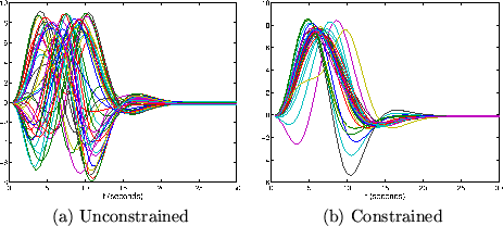 |
Figure 16:
Samples from the marginal posterior of the HRF at a
single voxel which is strongly activating in the pain experiment.
(a) Unconstrained with and (b) Constrained with
and
 |
Next: Discussion
Up: FMRI data
Previous: Methods