Results

The results are shown in table 1. It can be seen that even for the boxcar design, colouring is not as efficient as variance correction or prewhitening. For the randomized ISI design, the contrast is even more apparent, with prewhitening being more efficient than variance correction, which in turn is much more efficient than colouring. This concurs with the theory and work by Friston et al. (2000).

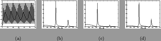
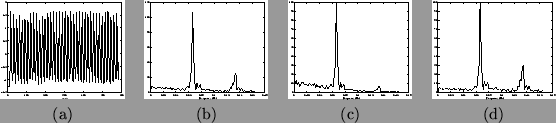
Examination of the spectral density for the randomized ISI design before and after it has been low-pass filtered (when colouring) illustrates the reason for the loss in efficiency. These spectra are shown in figures 10(b) and (c) respectively. It might have been expected that the frequency response in figure 10(b) would have relatively little high frequency content due to convolution with the smooth HRF whose spectral density is shown in figure 6(b). However, there are clearly strong high frequency components in the regressor. These are introduced when the high temporal resolution version of the regressor is sampled to a lower temporal resolution. Figure 10(c) clearly shows a reduction in these high frequency components due to the low pass filtering, resulting in a loss of efficiency. In contrast, comparing figure 7(b) with figure 7(c) reveals little difference particularly with regard to most of the power being in the fundamental frequency. Hence for the boxcar, colouring has similar efficiency to variance correction and prewhitening.

However, this does not explain why variance correction is less efficient than prewhitening for the randomized ISI design. This loss in efficiency is instead due to using a more inefficient estimator when using variance correction, compared with the best linear unbiased estimator (BLUE) of prewhitening. Here, the prewhitening down-weights the low frequencies compared to the high frequencies (inverse of figure 5) to give the BLUE. This is of particular benefit when the regressor has substantial power across a larger range of frequencies being weighted, such as is the case for the randomized ISI design (compare figure 10(b) with 10(d))

Figure: Plots of (a) the regressor $\mathbf{X}$ (b) the spectral density of $\mathbf{X}$ (c) the spectral density of $\mathbf{SX}$ where $\mathbf{S}$ is the colouring low-pass filtering Toeplitz matrix (d) the spectral density of $\mathbf{K^{-1}X}$ where $\mathbf{K^{-1}}$ is the prewhitening matrix from $\mathbf{V=KK^T}$. Where $\mathbf{X}$ is a boxcar.

Figure: As for figure 7, but $\mathbf{X}$ is a single-event design with fixed ISI.

Figure: As for figure 7, but $\mathbf{X}$ is a single-event design with jittered ISI.

Figure: As for figure 7, but $\mathbf{X}$ is a single-event design with randomized ISI.

Table 1: Table showing relative efficiency $E$ (equation 20) calculated using the three different strategies for dealing with the autocorrelation and for four different types of regressor.

	boxcar	SE/fixed ISI	SE/jittered ISI	SE/random ISI
Colouring(eq.6)	0.96	0.70	0.68	0.21
Variance correction(eq.7)	0.99	0.98	0.98	0.80
Prewhitening(eq.8)	1.00	1.00	1.00	1.00