|
After estimating the mixing-matrix
![]() , the source estimates are
calculated according to equation 6 by projecting each voxel's time
course onto the time courses contained in the columns of the unmixing matrix
, the source estimates are
calculated according to equation 6 by projecting each voxel's time
course onto the time courses contained in the columns of the unmixing matrix
![]() .
.
[McKeown et al., 1998] suggest transforming the spatial maps to ![]() -scores (transform the spatial maps to have zero mean and unit variance) and thresholding at
some level (e.g,
-scores (transform the spatial maps to have zero mean and unit variance) and thresholding at
some level (e.g, ![]() ). The spatial maps, however, are the result
of an ICA
decomposition where the estimation optimises for non-Gaussianity of the
distribution of spatial intensities. This is explicit in the case of the
fixed-point iteration algorithm employed here, but also true for the Infomax or
similar algorithms where the optimisation for non-Gaussian sources is implicit
in the choice of nonlinearity. As a consequence, the spatial
intensity histogram of an individual IC map is not Gaussian
and a simple transformation to voxel-wise
). The spatial maps, however, are the result
of an ICA
decomposition where the estimation optimises for non-Gaussianity of the
distribution of spatial intensities. This is explicit in the case of the
fixed-point iteration algorithm employed here, but also true for the Infomax or
similar algorithms where the optimisation for non-Gaussian sources is implicit
in the choice of nonlinearity. As a consequence, the spatial
intensity histogram of an individual IC map is not Gaussian
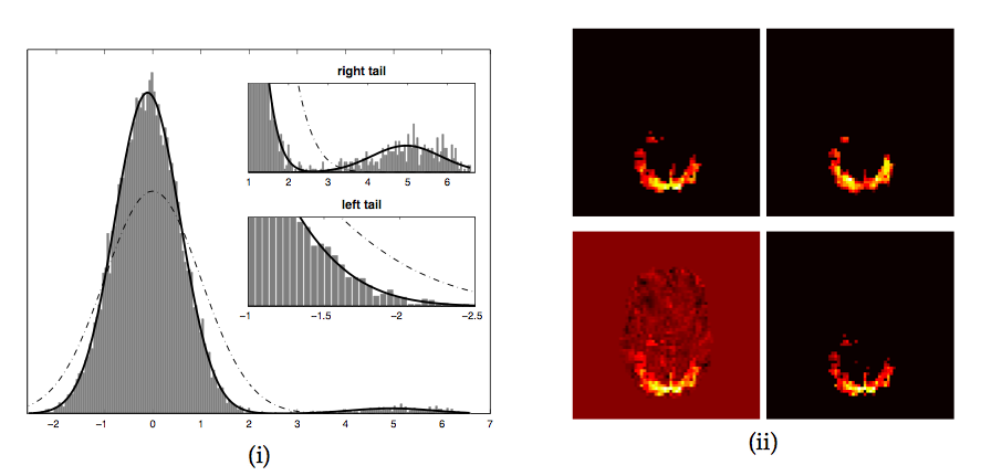
and a simple transformation to voxel-wise ![]() -scores and
subsequent thresholding will
necessarily result in an arbitrary and uncontrolled false-positive
rate:
the estimated mean and variance will not relate to an
underlying null-distribution. Figure 1 shows an
example where the estimated Gaussian (dash-dotted line) neither
represents the 'background noise' Gaussian nor the entire image
histogram, and any threshold value based on the expected number of
false-positives becomes meaningless with respect to the spatial map.
-scores and
subsequent thresholding will
necessarily result in an arbitrary and uncontrolled false-positive
rate:
the estimated mean and variance will not relate to an
underlying null-distribution. Figure 1 shows an
example where the estimated Gaussian (dash-dotted line) neither
represents the 'background noise' Gaussian nor the entire image
histogram, and any threshold value based on the expected number of
false-positives becomes meaningless with respect to the spatial map.
Instead, consider the estimated residual noise at a single voxel
location ![]() :
:
 is the residual
generating projection matrix. In the case where the model order
is the residual
generating projection matrix. In the case where the model order Under the null-hypothesis of no signal and after variance-normalisation, the estimated sources are just random regression coefficients which, after this transformation, will have a clearly defined and spatially stationary voxel-wise false-positive rate at any given threshold level.3While, for reasons outlined above, the null-hypothesis test is generally not appropriate, the voxel-wise normalisation also has important implication under the alternative hypothesis; it normalises what has been estimated as effect (the raw IC maps) relative to what has been estimated as noise and thus makes different voxel locations comparable in terms of their signal-to noise characteristics for a now given basis (the estimated mixing matrix). This is important since the mixing matrix itself is data- driven. As such, the estimated mixing matrix will give a better temporal representation at different voxel locations than at others and this change in 'specificity' is reflected in the relative value of residual noise.
In order to assess the ![]() -maps for significantly activated voxels, we follow
[Everitt and Bullmore, 1999] and [Hartvig and Jensen, 2000] and employ mixture modelling of the
probability density for spatial map of
-maps for significantly activated voxels, we follow
[Everitt and Bullmore, 1999] and [Hartvig and Jensen, 2000] and employ mixture modelling of the
probability density for spatial map of ![]() -scores.
-scores.
Equation 6 implies that
In cases where the number of 'active' voxels is small, however, a single
Gaussian mixture may actually have the highest model evidence, simply due to the
fact that the model evidence is only approximated in the current approach. In
this case, however, a transformation to spatial ![]() -scores and subsequent
thresholding is appropriate, i.e. reverting to null hypothesis testing instead
of the otherwise preferable alternative hypothesis testing.
-scores and subsequent
thresholding is appropriate, i.e. reverting to null hypothesis testing instead
of the otherwise preferable alternative hypothesis testing.
If the mixture model contains more than a single Gaussian, we can calculate the
probability of any intensity value being background noise by evaluating the
probability density function of the single Gaussian that models the density of
background noise. Conversely, we can evaluate the set of
additional Gaussians and calculate the probability under the alternative
hypothesis of 'activation'4 with respect to the associated time course, i.e. we obtain the estimate of the posterior probability for activation of
voxel ![]() in the
in the ![]() -score map
-score map ![]() as [Everitt and Bullmore, 1999]:
as [Everitt and Bullmore, 1999]:
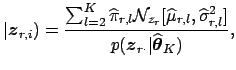
Figure 3 illustrates the process for a spatial map extracted from a data set with artificial activation introduced into FMRI resting data (see section 5 for details). Voxels with an estimated posterior probability of activation exceeding a certain threshold value are labeled active. The threshold level, though arbitrary, directly relates to the loss function we like to associate with the estimation process, e.g. a threshold level of 0.5 places an equal loss on false positives and false negatives [Hartvig and Jensen, 2000]. Alternatively, because we have explicitly modelled the probabilities under the null and alternative hypothesis, we can choose a threshold level based on the desired false positive rate over the entire brain or at the cluster level simply by evaluating the probabilities under the null and alternative hypotheses.
![$\displaystyle _K)=\sum_{l=1}^K \pi_{r,l}{\cal{N}}_{z_r}[\mu_{r,l},\sigma^2_{r,l}],$](img183.png)