(21) and (25) have previously used a
Bayesian framework to model epochs of the haemodynamic response to
a sustained period of stimulation. The advantage of a Bayesian
approach is most obvious in the use of prior experience to justify
the prior distributions used for these haemodynamic response
parameters.
To allow modelling of BOLD responses to general stimulation
types, (18) introduced the use of convolution models
assuming a linear time invariant system. (5),
(7), (2) and (30) provide some
evidence that the BOLD response possesses linear characteristics
with respect to the stimulation. However, non-linearities are
predominant when there are short separations (less than
approximately 3 seconds) between stimuli (15). An
additional assumption is that the stimulus represents the
underlying neural activity. The stimulus (or neural activity) is
then convolved with the assumed or modelled HRF to give the
assumed BOLD response.
In (11) and (33) HRF models, which are
allowed to vary spatially, are considered within the framework of
the linear model. Straightforward attempts to allow variation in
parameterised forms would be nonlinear, preventing the use of the
convenient linear modelling approach. To avoid this problem,
variability in the HRF is introduced via basis sets.
In (9) an interesting empirical Bayes
approach is taken to HRF modelling with basis functions, whereby
the HRF (and other parameters) within a dataset are
probabilistically constrained by datasets from multiple sessions
and multiple subjects, by inferring on a hierarchical model which
incorporates all of the datasets. Basis sets specify a subspace in
which a particular HRF either lies or does not. This represents a
hard constraint and often the extent of the constraint is
difficult to control and/or interpret. (25) make the
point that in this regard using Bayesian prior information is
preferable to a basis set approach. Bayesian modelling offers the
possibility of soft constraints.
In addition, unlike basis functions, a nonlinear parameterised HRF
approach (that the Bayesian framework makes possible), allows
interpretation of the parameters in terms of HRF shape
characteristics directly. Furthermore, null hypothesis testing in
a frequentist framework with basis functions, requires the overall
effect for an underlying stimulus of interested to be tested for
using f contrasts. These mean that the directionality of the test
is lost - something which is very often of interest in FMRI
experiments. For these reasons we present a Bayesian approach to
linear HRF modelling for general stimuli using a novel
parameterisation of the HRF with interpretable parameters.
Our proposed form for the HRF is based on observed BOLD
responses (23). This consists of a main response
corresponding to an increase in the signal, and a dip in signal
before and after the larger increase in signal, possibly
reflecting a temporary imbalance between the metabolic activity
and blood flow. The dip after the main response is now widely
supported, whereas the existence of the early dip as a general
phenomenon is still debated.
One possibility would be to use an addition of Gaussians (35).
However,
there are a couple of problems evident with a Gaussian HRF model.
Firstly, the HRF is not forced to be zero at time . Clearly,
this does not reflect what we know physically. This is usually
overcome using Gamma functions instead of Gaussians.
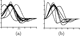
Figure 1:
11 evenly spread samples from the prior of the HRF, using
(a) two Gaussian model, and (b) the half-cosine HRF model.
The prior mean HRF is plotted along with different
HRFs each of which have one
parameter varying at the
percentile of the prior,
with the other parameters held at the mean prior
values.
The second problem is illustrated by Figure
1(a). This shows an evenly spread 11
samples of the HRF, taken from a sensible 5-dimensional prior
probability space. The problem is that there is dependence between
some of the HRF characteristics. It is difficult to interpret
characteristics when more than one distinct combinations of
parameters can affect them. This would also be a problem with the
two-parameter Gamma HRF. The clearest example of this problem is
the size of the post-stimulus undershoot. It is clear that the
post stimulus undershoot size could be affected by a number of
different combinations of parameters. Hence, this makes any
attempts to investigate undershoot difficult to perform.
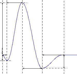
A solution to both of these problems is to use an alternative
parameterisation of the HRF. The one we present here is simply the
addition of four half-period cosines. There are six parameters;
four are the periods of the four cosines, and the other two are
the ratio of the height of the post-stimulus undershoot to the
height of the main peak and the ratio of the height of the initial
dip to the height of the main peak. Figure
2 shows a schematic of how the HRF is
parameterised.
Figure 2:
Parameterisation of the HRF into four half-period
cosines. There are six parameters.
Figure 1(b) shows an evenly spread 11
samples of the HRF without an initial dip ( and
), taken from the resulting 4 dimensional prior
probability space using the half-cosine HRF model.
A disadvantage with this parameterisation is that its second derivative
is discontinuous. However, the range of the HRF parameters are such
that sharp transitions in the second derivative are avoided. Hence,
sensible looking HRF shapes predominate, as illustrated by
figure 1(b).
This parameterisation does
clearly impose the constraint that the HRF is zero at .
Furthermore, parameters relating to HRF characteristics are independent. As
with the Gaussian HRF, another big advantage of the half-cosine
HRF model is that it could be parameterised in the frequency
domain, hence speeding up the convolution.
When figure 1(b) is compared
with figure 1(a), it can be seen how a
characteristic of the HRF shape, such as the size of the
undershoot, is now controlled by a single parameter.
Subsections