


Next: Inference
Up: Model
Previous: Choosing a Basis Set
Determining Basis Set
Constraints
In section 2.5 we determined a basis set to use. In
this section we describe how we can apply constraints on the
linear combinations of the basis set. In previous
work Friman et al. (2003) also looked to constrain the possible linear
combinations of the basis set, but within the canonical
correlation analysis framework. However, they only looked to
constrain the linear combination coefficients to be positive. In
this work we look to apply a more complete constraint by fitting a
multivariate Normal distribution to describe the desired
constrained space probabilistically within the GLM framework.
To date, basis sets are used by convolving the constituent basis
functions with the known stimulus to give the same number of
regressors as there are basis functions stimuli. The resulting
regressors are then used in the linear model. This approach
corresponds to the model we have described earlier but with  and
and  in equation 13.
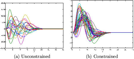
Figure 4(a) shows example HRF shapes obtained
randomly drawn from this basis set when the linear combinations
are unconstrained (i.e. with and ). If we compare these
HRFs with those in figure 2, it is clear
that unconstrained linear combinations of our basis set allows for
nonsensical HRF shapes.
To provide constraints on the possible linear combinations, we
regress the HRF samples we used to obtain our basis set back onto
the basis set:
in equation 13.
Figure 4(a) shows example HRF shapes obtained
randomly drawn from this basis set when the linear combinations
are unconstrained (i.e. with and ). If we compare these
HRFs with those in figure 2, it is clear
that unconstrained linear combinations of our basis set allows for
nonsensical HRF shapes.
To provide constraints on the possible linear combinations, we
regress the HRF samples we used to obtain our basis set back onto
the basis set:
 |
|
|
(15) |
where  is the
 matrix containing our
  HRF
samples,
HRF
samples,  is the
 matrix of our
  basis
functions and
basis
functions and
 . We can perform standard
Ordinary Least Squares (OLS) to obtain an estimate of the
. We can perform standard
Ordinary Least Squares (OLS) to obtain an estimate of the
 matrix,
  :
:
 |
|
|
(16) |
We then fit a -dimensional multivariate Normal distribution,
 , to the matrix
  . The
parameters of this multivariate Normal distribution are used to
set the parameters in equation 13 (i.e.
. The
parameters of this multivariate Normal distribution are used to
set the parameters in equation 13 (i.e.
 and
and
 ).
Using the HRF parameter value probabilities in
equation 14 for our half-cosine HRF
parameterisation,
).
Using the HRF parameter value probabilities in
equation 14 for our half-cosine HRF
parameterisation,  resulting HRF samples, and the resulting
top three eigenHRFs, we obtain the multivariate Normal
distribution parameters:
resulting HRF samples, and the resulting
top three eigenHRFs, we obtain the multivariate Normal
distribution parameters:
Figure 4(b) shows example HRF shapes obtained
randomly drawn from this basis set when the linear combinations
are constrained with these
and
. We can
see that compared with figure 4(a) this is a much
more faithful representation of the sensible HRF shapes in
figure 2.
It is important to point out that constraining the linear
combinations by using a multivariate Normal distribution is an
approximation. This is because a multivariate Normal will not
capture all of the detail of the distribution in the
parameter space. As figure 4(b) shows, whilst we
are producing much more sensible shapes than the unconstrained
case, there are still some undesirable HRF shapes. The alternative
is a fully parametric HRF approach (Woolrich et al., 2004b), which is
very slow to infer upon, or a different distribution to a
multivariate Normal which can capture the required detail in the
parameter space. However, we choose to use a multivariate
Normal as it will make inference much more easy to handle within
the Variational Bayesian framework, and it does capture the
required structure.
Figure 4:
Samples from the basis set: (a) unconstrained with
and , (b) constrained with
and
.
 |
Next: Inference
Up: Model
Previous: Choosing a Basis Set
![$\displaystyle \left[\! \begin{array}{ccc} 0.018 & 0.028 & -0.015 \\
0.028 & 0.185 & -0.009\\
-0.015 & -0.009 & 0.030
\end{array}\! \right]$](img126.png)