


Next: FCA-modes and FCA-modes
Up: -modes Correspondence Analysis
Previous: -modes Correspondence Analysis
Correspondence analysis of a two-way contingency table with cells
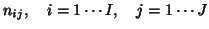 can be described as follows. The usual notations are:
and then the observed proportions
are defined as
 . Diagonal metrics containing vector margins
 and
and  used thereafter are noted
  and
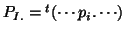
and  . Correspondence analysis
provides a decomposition of the measure of lack of independence between the two categorical
variables indexed respectively by
. Correspondence analysis
provides a decomposition of the measure of lack of independence between the two categorical
variables indexed respectively by  and
and  in performing the PCA (or generalised PCA) of the
following triple ([5]):
in performing the PCA (or generalised PCA) of the
following triple ([5]):
 |
(21) |
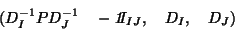
where the triple is defined as ( data, metric on  , metric on
  ). The
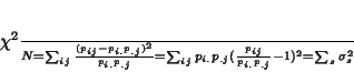
measure of lack of independence can be written :
). The
measure of lack of independence can be written :
 |
(22) |
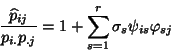
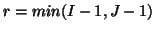
where the  are the singular values of the PCA of the triple given above. From the data
reconstruction formula, one can write for
are the singular values of the PCA of the triple given above. From the data
reconstruction formula, one can write for
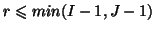 :
:
 |
(23) |
or equivalently in a tensor form:
 |
(24) |
where  ,
,
 , and
, and
 . If
. If
 the approximation is exact i.e.
  is
is  . From equation (24) and
 (which implies the solution
  ) it is possible to perform the PCA of the
triple:
) it is possible to perform the PCA of the
triple:
 |
(25) |
This last equation generalised for  enables to look at lack of marginal independence through
associated solutions of the first Principal Tensor ([10]).
enables to look at lack of marginal independence through
associated solutions of the first Principal Tensor ([10]).
Next: FCA-modes and FCA-modes
Up: -modes Correspondence Analysis
Previous: -modes Correspondence Analysis
Didier Leibovici
2001-09-04