


Next: Estimation of Forman et
Up: Estimation of Kiebel et
Previous: Estimating the Derivative
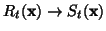
In practice the smoothness is estimated using the following steps:
- Normalise the 4D residuals,
 ,
using equation 37.
,
using equation 37.
- Calculate the derivative approximation
 at all 4D samples
using equation 40.
at all 4D samples
using equation 40.
- Calculate the 4D average statistic
 using
equation 39.
using
equation 39.
- Accumulate the results of
 into a matrix (assuming
non-diagonal elements are zero):
into a matrix (assuming
non-diagonal elements are zero):
 |
(41) |
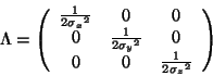
- Optional: Calculate the filter width matrix
 and the
FWHM values as
and the
FWHM values as
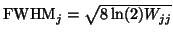 .
.
Mark Jenkinson
2001-11-07