


Next: HMRF-EM Framework for Brain
Up: Segmentation of Brain MR
Previous: Segmentation of Brain MR
One of the most successful methods for dealing with the bias field
problem was developed by Wells et al. [31], in
which the bias field
 is modelled as a
multiplicative N-dimensional random vector with zero mean
Gaussian prior probability density
is modelled as a
multiplicative N-dimensional random vector with zero mean
Gaussian prior probability density
 ,
where
,
where
 is the
 covariance matrix. Let
 and
and
 be the
observed and the ideal intensities of a given image respectively.
The degradation effect of the bias field at pixel
be the
observed and the ideal intensities of a given image respectively.
The degradation effect of the bias field at pixel
 can be expressed as follows:
 |
(29) |
After logarithmic transformation of the intensities, the bias
field effect can be treated as an additive artifact. Let
y and
y* denote respectively the observed and the
ideal log-transformed intensities: then
y =
y* + B. Given the class labels x, it is further
assumed that the ideal intensity value at pixel i follows a
Gaussian distribution with parameter
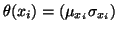 :
:
 |
(30) |
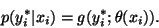
With the bias field bi taken into account, the above
distribution can be written in terms of the observed intensity
yi as
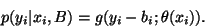 |
(31) |
Thus, the intensity distribution is modelled as a Gaussian
mixture, given the bias field. It follows that
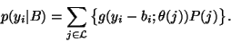 |
(32) |
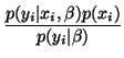
The MAP principle is then employed to obtain the optimal estimate
of the bias field, given the observed intensity values:
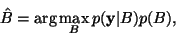 |
(33) |
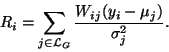
A zero-gradient condition is then used to assess this maximum,
which leads to (see [31] for detail):
| Wij |
= |
 |
(34) |
| bi |
= |
![$\displaystyle \frac{[FR]_i}{[F\psi^{-1}1]_i}, \text{ with }
1=(1,1,\cdots,1)^T,$](img129.gif) |
(35) |
where R is the mean residual for pixel i
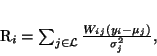 |
(36) |
 is the mean inverse covariance
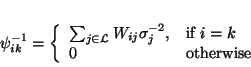 |
(37) |
and F is a lowpass filter. Wij is the posterior probability
that pixel i belongs to class j given the bias field estimate.
The EM algorithm is applied to Equations (34) and
(35). The E step assumes that the bias field is
known and calculates the posterior tissue class probability
Wij. In the M step, the bias field B is estimated given the
estimated Wij in the E step. Once the bias field is obtained,
the original intensity I* is restored by dividing I by the
inverse log of B. Initially, the bias field is assumed to be
zero everywhere.
Wells et al.'s algorithm is found to be problematic when
there are classes in an image that do not follow a Gaussian
distribution. The variance of such a class tends to be very large
and consequently the mean can not be considered
representative[13]. Such situations are commonly
seen in the regions of CSF, pathologies and other non-brain
classes. Bias field estimation can be significantly affected by
this type of problem. To overcome this problem, Guillemaud and
Brady [13] unify all such classes into an outlier
class, which is called ``other'', with uniform distribution. Let
 denote the set of labels for Gaussian classes and
lo the class label for the ``other'' class. The intensity
distribution of the image is still a finite mixture except with an
additional non-Gaussian class,
denote the set of labels for Gaussian classes and
lo the class label for the ``other'' class. The intensity
distribution of the image is still a finite mixture except with an
additional non-Gaussian class,
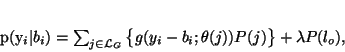 |
(38) |
where  is the density of the uniform distribution. Due to
the large variance of the uniform distribution, the bias field is
only estimated with respect to the Gaussian classes. The same
iterative EM method can be applied, except for a slight
modification to the formulation of mean residual Ri
(36)
is the density of the uniform distribution. Due to
the large variance of the uniform distribution, the bias field is
only estimated with respect to the Gaussian classes. The same
iterative EM method can be applied, except for a slight
modification to the formulation of mean residual Ri
(36)
 |
(39) |
With such a modification, the performance of the EM algorithm can
be significantly improved in certain situations. This approach is
referred to as the modified EM (MEM) algorithm.
Next: HMRF-EM Framework for Brain
Up: Segmentation of Brain MR
Previous: Segmentation of Brain MR
Yongyue Zhang
2000-05-11