Experiments

Various experiments have been carried out both on real and simulated data, in both 2D and 3D. For the MEM algorithm, the parameters used in the experiments take their actual values for the simulated images and are manually estimated for real data, since the algorithm does not deal with parameter estimation itself. For the HMRF-EM algorithm, parameters are estimated automatically. The first experiment shown here tests the noise sensitivity of the two algorithms. Two images consisting of two constant regions with the same simulated bias field but with different white noise were generated (Figure 6(a),(b)). Two Gaussian classes, corresponding to the two regions, are used. For Figure 6(a), both algorithms give perfect estimation results, as shown in Figures 6(c) and (d). However, for Figure 6(b), the HMRF-EM algorithm gives much better results than the MEM algorithm.

  

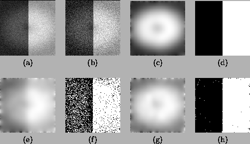
Figure 6: Comparison of the MEM and the HMRF-EM algorithm on simulated 2D images. (a) the original image with 3% noise. (b) the original image with 10% noise. (c) bias field estimation for (a) by both the algorithms. (d) segmentation for (a) by both the algorithms. (e) bias field estimation for (b) by the MEM algorithm. (f) segmentation for (b) by the MEM algorithm. (g) bias field estimation for (b) by HMRF-EM algorithm. (h) segmentation for (b) by the HMRF-EM algorithm.

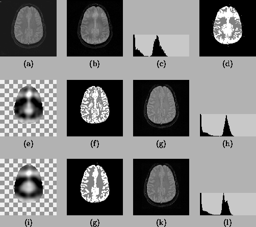
The second experiment tests the performance of the two algorithms on real 2D MR images but with a simulated bias field. Two Gaussian distributions are used for the two tissue classes (white matter and grey matter) and a uniform distribution (density = 0.3) is used for the rest. Figure 7(a) is the original T₂-weighted image and Figure 7(b) is the image with a simulated circular bias field. Figure 7(c) is the histogram of Figure 7(b), from which a substantial intensity overlap between WM and GM can be seen. Figure 7(d) shows the best result that can be obtained from (a) using global thresholding. The second row shows the result of applying the MEM algorithm. The last row shows the results from the HMRF-EM algorithm. Comparing the segmentations, we see that without losing any significant structure, the results from the HMRF-EM algorithm are much cleaner than from the MEM method, which still looks noisy. The restored image from HMRF-EM algorithm also shows good intensity uniformity, while the histogram output in the MEM method still shows WM/GM overlap.

  

Figure 7: Comparison of the MEM and the HMRF-EM algorithm on real 2D MR images with simulated bias field. (a) the original image; (b) the image with simulated bias field; (c) histogram of (b); (d) best thresholding on (b); (e)-(h) the results from the MEM algorithm; (i)-(l) the results from HMRF-EM algorithm. For the last two rows, from left to right: the estimated bias field (the checkerboard is used to represent the background which is assumed to have no bias field), the segmentation, the restored image and the histogram of the restored image.

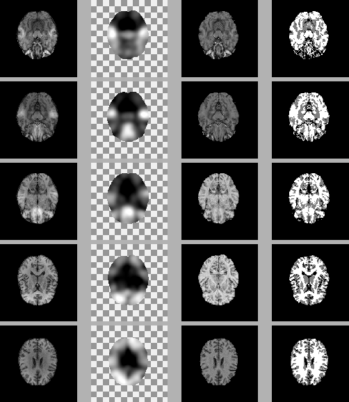
The last example we show is for a real 3D data set from the Montreal Neurological Institute, McGill University, courtesy of D. Arnold. The original volume has 50 $256\times 256$ slices with voxel size $0.977\times 0.977\times 3.0$ mm. Figure 8 shows the results of five different slices from the HMRF-EM algorithm.

  

Figure 8: Five slices of a 3D MR volume image with real bias field. In each row, from left to right: the original slice, the estimated bias field, the restored slice, and the segmentation.