Appendix

The general form of the Sherman-Morrison-Woodbury formula [8] is

$$\left( A + B C D \right)^{\mbox{\scriptsize\textit{\sffamily {-1}... ...ptsize\textit{\sffamily {-1}}}}D A^{\mbox{\scriptsize\textit{\sffamily {-1}}}}.$$ (18)

Also, the inverse for a matrix in block form is given by

$$\left[ \begin{array}{cc} A & B \\ B^{\mbox{\scriptsize\textit{\sf... ...1}}}}B \right)^{\mbox{\scriptsize\textit{\sffamily {-1}}}} \end{array} \right].$$

Theorem A:

Any model of the form

$$Y = \left[ X_1 \; \; Z_1 \right] \left[ \begin{array}{c} \beta_1 \\ \alpha_1 \end{array} \right] + \epsilon$$

can be rewritten as

$$Y = \left[ X_2 \; \; Z_2 \right] \left[ \begin{array}{c} \beta_2 \\ \alpha_2 \end{array} \right] + \epsilon,$$

where $Z_2^{\mbox{\scriptsize\textit{\sffamily {$\!$T}}}}V^{\mbox{\scriptsize\textit{\sffamily {-1}}}}X_2 = 0$ whilst being completely equivalent in terms of the estimated parameters of interest ( $\widehat{\beta_2} = \widehat{\beta_1} \; , \; \textrm{Cov}(\widehat{\beta_2}) = \textrm{Cov}(\widehat{\beta_1})$) and the modelled signal space: $\textrm{Span}(X_2) \, \cup \, \textrm{Span}(Z_2) = \textrm{Span}(X_1) \, \cup \, \textrm{Span}(Z_1)$ in the pre-whitened space. Note that $\textrm{Cov}(\epsilon) = V$ for both models.

That is, the signals of interest can be made orthogonal to the confounds without affecting the estimation of the parameters or the residuals.

Proof:

The proof is by construction, where we show that orthogonalising $X_1$ with respect to $Z_1$ gives the desired results. Let

$$X_2 = X_1 - P_{Z_1} X_1 %% = X_1 - Z_1 ( Z_1\T V\inv Z_1)\inv Z_1\T V\inv X_1 \quad \textrm{and} \quad Z_2 = Z_1$$

where $P_{Z_1} = Z_1 ( Z_1^{\mbox{\scriptsize\textit{\sffamily {$\!$T}}}}V^{\mbox{\sc... ...ptsize\textit{\sffamily {$\!$T}}}}V^{\mbox{\scriptsize\textit{\sffamily {-1}}}}$ is the projection matrix for $Z_1$ in the pre-whitened space.

These equations give $Z_2^{\mbox{\scriptsize\textit{\sffamily {$\!$T}}}}V^{\mbox{\scriptsize\textit{... ...}}V^{\mbox{\scriptsize\textit{\sffamily {-1}}}}({\mathbf {I}}- P_{Z_1}) X_1 = 0$. Also, the combined span of $X_2$ and $Z_2$ is clearly the same as that of $X_1$ and $Z_1$.

Now consider the covariances

$$\textrm{Cov}\left(\left[ \!\! \begin{array}{c} \widehat{\beta_1} ... ... D \end{array} \! \right]^{\mbox{\scriptsize\textit{\sffamily {-1}}}}\!\!\!\!.$$

Using the block matrix inverse, this gives

$$\textrm{Cov}(\widehat{\beta_1}) = \left(A - B D^{\mbox{\scriptsize\textit{\sffamily {-1}}}}B^{\mbox... ...textit{\sffamily {$\!$T}}}}\right)^{\mbox{\scriptsize\textit{\sffamily {-1}}}},$$

while, since the off-diagonal blocks are zero in the second case, the calculation simply gives

$$\textrm{Cov}(\widehat{\beta_2}) = (X_2^{\mbox{\scriptsize\textit{\sffamily {$\!$T}}}}V^{\mbox{\scriptsize\textit{\sffamily {-1}}}}X_2)^{\mbox{\scriptsize\textit{\sffamily {-1}}}}$$

$$= \left\{ (X_1^{\mbox{\scriptsize\textit{\sffamily {$\!$T}}}}- B D^... ...xtit{\sffamily {$\!$T}}}}) \right\}^{\mbox{\scriptsize\textit{\sffamily {-1}}}}$$

$$= \left( A - B D^{\mbox{\scriptsize\textit{\sffamily {-1}}}}B^{\mbo... ...\textit{\sffamily {$\!$T}}}}\right)^{\mbox{\scriptsize\textit{\sffamily {-1}}}}$$

$$= \textrm{Cov}(\widehat{\beta_1}).$$

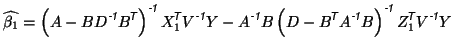
For the first model, the parameter estimates, given by equation 5, can be written using the matrix block inversion formula, giving

$$\widehat{\beta_1} =\left( A - B D^{\mbox{\scriptsize\textit{\sffa... ...tsize\textit{\sffamily {$\!$T}}}}V^{\mbox{\scriptsize\textit{\sffamily {-1}}}}Y$$ (19)

while for the second model, the block diagonal form yields the familiar form

$$\widehat{\beta_2} = (X_2^{\mbox{\scriptsize\textit{\sffamily {$\!$T}}}}V^{\mbox{\scri... ...tsize\textit{\sffamily {$\!$T}}}}V^{\mbox{\scriptsize\textit{\sffamily {-1}}}}Y$$

$$= \textrm{Cov}(\widehat{\beta_2}) \left( X_1^{\mbox{\scriptsize\tex... ...tit{\sffamily {$\!$T}}}}V^{\mbox{\scriptsize\textit{\sffamily {-1}}}}\right) Y.$$

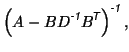
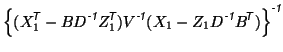
Applying the Sherman-Morrison-Woodbury formula to the second term in equation 12 gives

$$A^{\mbox{\scriptsize\textit{\sffamily {-1}}}}B \left( D - B^{\mbo... ...e\textit{\sffamily {-1}}}}B \right)^{\mbox{\scriptsize\textit{\sffamily {-1}}}} = A^{\mbox{\scriptsize\textit{\sffamily {-1}}}}\left( {\mathbf {I}}... ...textit{\sffamily {-1}}}}\right) B D^{\mbox{\scriptsize\textit{\sffamily {-1}}}}$$

$$= (A - B D^{\mbox{\scriptsize\textit{\sffamily {-1}}}}B^{\mbox{\scr... ...iptsize\textit{\sffamily {-1}}}}B D^{\mbox{\scriptsize\textit{\sffamily {-1}}}}$$

$$= \textrm{Cov}(\widehat{\beta_1}) B D^{\mbox{\scriptsize\textit{\sffamily {-1}}}}.$$

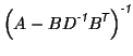
Substituting this into equation 12 gives

$$\widehat{\beta_1} = \textrm{Cov}(\widehat{\beta_1}) \left( X_1^{\mbox{\scriptsize\tex... ...xtit{\sffamily {$\!$T}}}}V^{\mbox{\scriptsize\textit{\sffamily {-1}}}}Y \right)$$

$$= \widehat{\beta_2}$$

$\Box$

Theorem B:

Given the standard GLM, $Y = X\beta + \epsilon$, and a set of linearly independent contrasts specified by $C_1$ such that $\widehat{b_1} = C_1^{\mbox{\scriptsize\textit{\sffamily {$\!$T}}}}\widehat{\beta}$, then an equivalent model without contrasts, but with confounds, exists in the form

$$Y = \left[ X_2 \; \; Z_2 \right] \left[ \begin{array}{c} b \\ \alpha \end{array}\right] + \epsilon.$$

That is, $\widehat{b} = C_1^{\mbox{\scriptsize\textit{\sffamily {$\!$T}}}}\widehat{\beta}$, $\textrm{Cov}(\widehat{b}) = C_1^{\mbox{\scriptsize\textit{\sffamily {$\!$T}}}}\textrm{Cov}(\widehat{\beta}) C_1$ and the modelled signal space: $\textrm{Span}(X_2) \, \cup \, \textrm{Span}(Z_2) = \textrm{Span}(X)$ in the pre-whitened space. Note that $\textrm{Cov}(\epsilon) = V$ for both models.

Proof:

The proof is, again, by construction. Firstly, let $C_2$ be a set of contrasts that when combined with $C_1$ form a complete linearly independent set of contrasts. That is, the matrix $C = [ C_1 \; \; C_2 ]$ will be full rank (and hence invertible). Then let

$$X_2 = X Q C_1 F_1 \quad \textrm{and} \quad Z_2 = X Q C_3 F_3$$

where

$$Q = (X^{\mbox{\scriptsize\textit{\sffamily {$\!$T}}}}V^{\mbox{\sc... ...textit{\sffamily {$\!$T}}}}Q C_3)^{\mbox{\scriptsize\textit{\sffamily {-1}}}}.$$

From these definitions it is easy to see that $C_1^{\mbox{\scriptsize\textit{\sffamily {$\!$T}}}}Q C_3 = 0$, which represents an orthogonality condition. As before, it is straightforward to verify that the combined span of $X_2$ and $Z_2$ is equal to the span of $X$. Consequently,

$$Z_2^{\mbox{\scriptsize\textit{\sffamily {$\!$T}}}}V^{\mbox{\scrip... ...C_1 F_1 = F_3 C_3^{\mbox{\scriptsize\textit{\sffamily {$\!$T}}}}Q C_1 F_1 = 0.$$

Therefore, $Z_2$ and $X_2$ are orthogonal as well.

The estimation equations for the model become

$$\textrm{Cov}\left(\left[ \begin{array}{c} \widehat{b} \\ \widehat{\alpha} \end{array} \right]\right) = \left[ \begin{array}{cc} (X_2^{\mbox{\scriptsize\textit{\sffamily... ...mily {-1}}}}Z_2)^{\mbox{\scriptsize\textit{\sffamily {-1}}}}\end{array}\right],$$

$$\left[ \begin{array}{c} \widehat{b} \\ \widehat{\alpha} \end{array} \right] = \left[ \begin{array}{c} (X_2^{\mbox{\scriptsize\textit{\sffamily ... ...y {$\!$T}}}}V^{\mbox{\scriptsize\textit{\sffamily {-1}}}}\end{array} \right] Y.$$

Thus

$$\textrm{Cov}(\widehat{b}) = \left(F_1 C_1^{\mbox{\scriptsize\textit{\sffamily {$\!$T}}}}Q X^{... ...\sffamily {-1}}}}X Q C_1 F_1\right)^{\mbox{\scriptsize\textit{\sffamily {-1}}}}$$

$$= \left(F_1 C_1^{\mbox{\scriptsize\textit{\sffamily {$\!$T}}}}Q C_1 F_1 \right)^{\mbox{\scriptsize\textit{\sffamily {-1}}}}$$

$$= F_1^{\mbox{\scriptsize\textit{\sffamily {-1}}}}= C_1^{\mbox{\scri... ...tsize\textit{\sffamily {-1}}}}X)^{\mbox{\scriptsize\textit{\sffamily {-1}}}}C_1$$

$$= C_1^{\mbox{\scriptsize\textit{\sffamily {$\!$T}}}}\textrm{Cov}(\widehat{\beta}) C_1$$

and

$$\widehat{b} = \textrm{Cov}(\widehat{b}) (F_1 C_1^{\mbox{\scriptsize\textit{\sff... ...ize\textit{\sffamily {$\!$T}}}}) V^{\mbox{\scriptsize\textit{\sffamily {-1}}}}Y$$

$$= C_1^{\mbox{\scriptsize\textit{\sffamily {$\!$T}}}}(Q X^{\mbox{\sc... ...ize\textit{\sffamily {$\!$T}}}}V^{\mbox{\scriptsize\textit{\sffamily {-1}}}}) Y$$

$$= C_1^{\mbox{\scriptsize\textit{\sffamily {$\!$T}}}}\widehat{\beta}$$

$\Box$