 ++++ PTA-  3 modes ++++
               data=  J12.gm16   576 100 12
    just slice 16
                ------Percent Rebuilt---- 23.34021%
                ------Percent Rebuilt from Selected ---- 17.01323%
                 -no- --Sing Val-- --ssX-- --local Pct-- --Global Pct--
vs111               1      191.376  599772        6.1064         6.1064
576 vs111 100 12    3       85.062   70189       10.3088         1.2064
100 vs111 576 12    6       97.382   81266       11.6694         1.5812
100 vs111 576 12    7       87.138   81266        9.3434         1.2660
12 vs111 576 100    9       87.616   80815        9.4988         1.2799
vs222              11      133.299  440752        4.0314         2.9625
vs333              21       97.991  370027        2.5950         1.6010
12 vs333 576 100   29       77.825   42284       14.3237         1.0098

 ++++               ++++
 Shown are selected over  21  PT  with var> 1% total
| ![\includegraphics[width=15cm]{rgm16.vs111.ps}](img18.gif)
![\includegraphics[width=15cm]{rgm16.vs222.ps}](img29.gif)
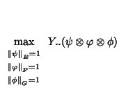
![$\displaystyle \max_{{\scriptstyle
\begin{array}{l }
\scriptstyle \left\Vert \va...
...\left\Vert \phi \right\Vert _G =1
\end{array}}}E([Y'..(\varphi \otimes \phi)]2)$](img20.gif)
![$\displaystyle \max_{{\scriptstyle
\begin{array}{l }
\scriptstyle \left\Vert \va...
...ray}}}E([Y'\otimes Y'])..([\varphi \otimes \phi]\otimes [\varphi \otimes \phi])$](img21.gif)
![$\displaystyle \max_{{\scriptstyle
\begin{array}{l }
\scriptstyle \left\Vert \va...
...
\end{array}}}E([Y'..\phi_1] \otimes [Y'..\phi_1]) .. (\varphi \otimes \varphi)$](img22.gif)
![$\displaystyle \max_{{\scriptstyle
\begin{array}{l }
\scriptstyle \left\Vert \ph...
...
\end{array}}}E([Y'..\varphi_1] \otimes [Y'..\varphi_1]) .. (\phi \otimes \phi)$](img23.gif)