Spatial Variation

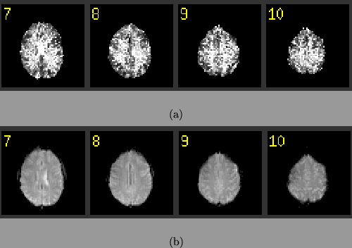
Figure 4 shows four slices of the $S_{\rho }$ values in the brain volume after non-linear high-pass filtering has been performed, along with the original functional image, for comparison.

Figure 4: (a) Spatial maps of $S_{\rho }$ in the brain volume after the non-linear high-pass filtering has been performed. This corresponds to the histogram in figure 3(b), with high $S_{\rho }$ displayed as lighter grey and low $S_{\rho }$ as darker grey. (b) EPI for the same slices. Exactly the same characteristic could be easily observed in five other null data sets.

Figure 4 shows considerable spatial variation and structure, with lower $S_{\rho }$ corresponding to increased autocorrelation in the grey matter compared to the white-matter and CSF. Exactly the same characteristic could be easily observed in five other null data sets.

These findings appear to contradict Zarahn's and Lund's conclusions that the autocorrelation is not at all physiological in origin. It may be that the greater smoothness in the grey-matter is due to a larger number of edges in grey-matter compared to white matter. Edges within voxels may be subject to motion of any type (inaccurate motion correction, physiological pulsations), and this motion along with a partial volume effect may produce increased low frequency noise. Further analysis is required to understand such sources of the autocorrelations that could exhibit these characteristics. This will be a topic for future research.