 |
Given the similarity of temporal autocorrelation in the local neighbourhood of each voxel, we attempt to improve the robustness of the autocorrelation estimates using a small amount of local spatial smoothing. However, our qualitative data analysis indicated clearly that the autocorrelation differs between tissue types. Isotropic spatial smoothing would blur the autocorrelation estimates across tissue boundaries, resulting in biased estimates of the autocorrelation near tissue boundaries. An alternative approach is to use some form of nonlinear spatial smoothing that does not smooth across such boundaries.
Accurate segmentation of white-matter, grey-matter and CSF would provide the necessary information to avoid blurring across tissue types. However, segmentation of EPI images is hard due to poor tissue type contrast, bias field effects, low resolution and the partial volume effect.
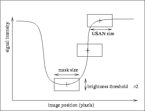
Instead we use the ``Smoothing over Univalue Segment Assimilating Nucleus'' (SUSAN) noise reduction filter (Smith and Brady, 1997), which is a nonlinear filter designed to preserve image structure by only smoothing over those neighbours which form part of what is believed to be the ``same region'', or USAN, as the central voxel under consideration. This concept is illustrated in 1-D in Figure 11.
 |
The filter averages over all the pixels in the locality which lie in the USAN using the weighting,
We can use a 3D version of this filter to spatially smooth the raw autocorrelation estimate at each lag or to spatially smooth the spectral density estimate at each frequency. Whether we smooth the autocorrelation or the spectral density estimates will depend upon the autocorrelation/spectral density estimation technique then used on the spatially regularised data.
Normally, the USAN is estimated from the same data, or image, as that which is being smoothed. However, here we will be using one of the EPI volumes to generate the USAN.
We would expect a ![]() of approximately 1 or 2 voxels to be optimal, since
the spatial autocorrelation of
of approximately 1 or 2 voxels to be optimal, since
the spatial autocorrelation of ![]() suggests that smoothness is
in the immediate neighbourhood only. Simple histogram
techniques are used to assess the approximate standard deviation
of grey matter in the EPI. The brightness threshold
suggests that smoothness is
in the immediate neighbourhood only. Simple histogram
techniques are used to assess the approximate standard deviation
of grey matter in the EPI. The brightness threshold ![]() is then set to
is then set to ![]() of the
approximate standard deviation of grey matter. This gives a very conservative
brightness threshold
of the
approximate standard deviation of grey matter. This gives a very conservative
brightness threshold ![]() , one which allows a small amount of smoothing
within grey matter whilst allowing negligible smoothing between matter types.
, one which allows a small amount of smoothing
within grey matter whilst allowing negligible smoothing between matter types.