Autocorrelation Spatial Smoothing

We have established that without any spatial regularisation of the autocorrelation estimate, the single taper Tukey with $M=5,10$ perform best. We now want to explore the additional benefits, if any, of using the SUSAN spatial smoothing of the raw autocorrelation estimate before the Tukey tapering is applied and also to establish how much smoothing is of benefit. Spatial autocorrelation of the $S_\rho$ map suggests that the autocorrelation is only correlated over a short range. The voxel dimensions for the 6 datasets are $4\times4\times7 mm$ and hence we consider SUSAN filtering with $\sigma_s=4,8,12 mm$.

Although the single taper Tukey performed better with $M=10$, because we are now regularising spatially, it turns out to be better to allow more flexibility (i.e. less smoothing) of the spectral density by choosing a Tukey taper with $M=15$. Figures 16 (TR=3 secs) and 17(b) (TR=1.5 secs) show the results of the different amounts of spatial smoothing. A $\sigma _s$ of $8mm$ performs best and shows improvement over performing no spatial smoothing for the TR=3 secs data and performs similarly for the TR=1.5 secs data.

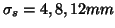
Figure 13: Comparison of Tukey autocorrelation estimation for different values of $M$ via log probability plots comparing theoretical $p$ against null distribution $p_{null}$ obtained from six different null datasets using TR=3 secs for (a) a boxcar design convolved with a gamma HRF, and (b) a stochastic single-event design convolved with a gamma HRF. All are calculated using prewhitening. The straight dotted line shows the result for what would be a perfect match between theoretical and null distribution.

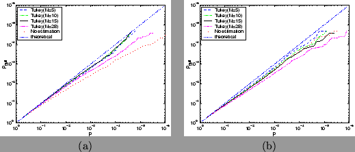Figure 14: Comparison of Multitapering autocorrelation estimation for different values of $NW$ via log probability plots comparing theoretical $p$ against null distribution $p_{null}$ obtained from six different null datasets using TR=3 secs for (a) a boxcar design convolved with a gamma HRF, and (b) a stochastic single-event design convolved with a gamma HRF. All are calculated using prewhitening. The straight dotted line shows the result for what would be a perfect match between theoretical and null distribution.

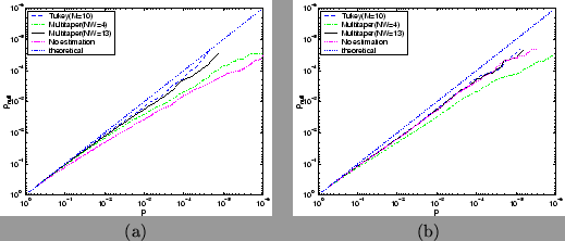Figure 15: Comparison of the different autocorrelation estimation techniques via log probability plots comparing theoretical $p$ against null distribution $p_{null}$ obtained from six different null datasets using TR=3 secs for (a) a boxcar design convolved with a gamma HRF, and (b) a stochastic single-event design convolved with a gamma HRF. All are calculated using prewhitening. The straight dotted line shows the result for what would be a perfect match between theoretical and null distribution.

Figure 16: Comparison of different amounts of spatial smoothing of the raw autocorrelation estimate prior to using Tukey tapering with $M=15$, via log probability plots comparing theoretical $p$ against null distribution $p_{null}$ obtained from six different null datasets using TR=3 secs for (a) a boxcar design convolved with a gamma HRF, and (b) a stochastic single-event design convolved with a gamma HRF. All are calculated using prewhitening. The straight dotted line shows the result for what would be a perfect match between theoretical and null distribution. MS is the mask-size used in the SUSAN smoothing and corresponds to $\sigma _s$.

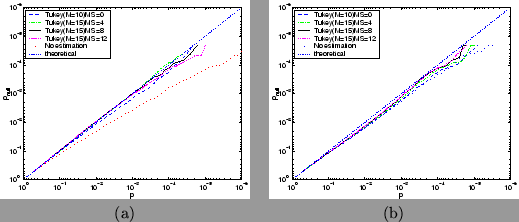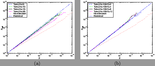
Figure 17: (a) Comparison of Tukey autocorrelation estimation for different values of $M$, and (b) Comparison of different amounts of spatial smoothing of the raw autocorrelation estimate prior to using Tukey tapering with $M=15$, for data taken with TR=1.5 secs. The comparison is made via log probability plots comparing theoretical $p$ against null distribution $p_{null}$ obtained from nine different null datasets with a stochastic single-event design convolved with a gamma HRF. All are calculated using prewhitening. The straight dotted line shows the result for what would be a perfect match between theoretical and null distribution. MS is the mask-size used in the SUSAN smoothing and corresponds to $\sigma _s$.