Bayesian Inference

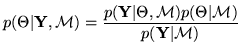
The two rules at the heart of Bayesian learning techniques are conceptually very simple. The first tells us how (for a model $\mathcal{M}$) we should use the data, $\mathbf{Y}$, to update our prior belief in the values of the parameters $\Theta$, $p(\Theta\vert\mathcal{M})$ to a posterior distribution of the parameter values $p(\Theta\vert\mathbf{Y},\mathcal{M})$. This is known as Bayes' rule:

$$p(\Theta\vert\mathbf{Y},\mathcal{M})= \frac{p(\mathbf{Y}\vert\Theta,\mathcal{M})p(\Theta\vert\mathcal{M})}{p(\mathbf{Y}\vert\mathcal{M})}$$ (4)

Unfortunately, calculating this posterior pdf is seldom straightforward. The denominator in equation 4 is:

$$p(\mathbf{Y}\vert\mathcal{M})=\int_{\Theta}p(\mathbf{Y}\vert\Theta,\mathcal{M})p(\Theta\vert\mathcal{M})d\Theta$$ (5)

an integral which is often not tractable analytically. To make matters worse, this joint posterior pdf on all parameters is often not the distribution which we are most interested in. We are often interested in the posterior pdf on a single parameter, or an interesting subset of parameters. Obtaining these marginal distributions again involves performing large integrals,

$$p(\Theta_I\vert\mathbf{Y},\mathcal{M})= \int_{\Theta_{-I}}p(\Theta\vert\mathbf{Y},\mathcal{M})d{\Theta_{-I}}$$ (6)

where $\Theta_I$ are the parameters of interest and $\Theta_{-I}$ are all other parameters. Again these integrals are seldom tractable analytically.

One solution is to use approximations to the marginal distributions. This is the approach we take in section 3.5. Another solution is to draw samples in parameter space from the joint posterior distribution, implicitly performing the integrals numerically. For example, we may repetitively choose random sets of parameter values and choose to accept or reject these samples according to a criterion based on the value of the numerator in equation 4. It can be shown (e.g (13)) that a correct choice of this criterion will result in the accepted samples being distributed according to the joint posterior pdf (equation 4). Schemes such as this are rejection sampling and importance sampling which generate independent samples from the posterior. Any marginal distributions may then be generated by examining the samples from only the parameters of interest. However, these kinds of sampling schemes tend to be very slow, particularly in high dimensional parameter spaces, as samples are proposed at random, and thus each has a very small chance of being accepted.

Markov Chain Monte Carlo (MCMC) (see (13) and (12) for texts on MCMC) is a sampling technique which addresses this problem by proposing samples preferentially in areas of high probability. Samples drawn from the posterior are no longer independent of one another, but the high probability of accepting samples, allows for many samples to be drawn and, in many cases, for the posterior pdf to be built in a relatively short period of time. This is the approach we take in section 3.6.