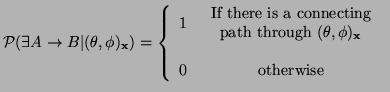
Consider the case where the values of the local parameters are known with no uncertainty. What do they tell us about anatomical connectivity between voxels in the brain? In the case where our local model describes only a single fiber direction passing through the voxel, this global model can only take one form:
Where
![]() is the probability of a connection existing between points
is the probability of a connection existing between points ![]() and
and
![]() , given knowledge of local fiber direction.
, given knowledge of local fiber direction.
In order to solve this equation we may simply start a connected path
from a seed point, ![]() , and follow local fiber direction until a
stopping criterion is met. If
, and follow local fiber direction until a
stopping criterion is met. If ![]() lies on this path we may say that
a connection exits between
lies on this path we may say that
a connection exits between ![]() and
and ![]() . This procedure is at the
heart of all ``streamlining'' algorithms
(e.g. [6,19,5]), which choose
. This procedure is at the
heart of all ``streamlining'' algorithms
(e.g. [6,19,5]), which choose
![]() to be the principal eigen-direction of the
estimated diffusion tensor at each voxel.
to be the principal eigen-direction of the
estimated diffusion tensor at each voxel.
However, in the case where there is uncertainty associated with
![]() we would like to compute the probability of
a connection existing given the data,
we would like to compute the probability of
a connection existing given the data,
![]() , which
is known. That is, we would like to compute
, which
is known. That is, we would like to compute
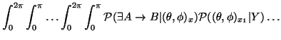
![]() . In order to calculate this pdf we would have to perform the following integrations:
. In order to calculate this pdf we would have to perform the following integrations:
That is, for each possible value of fiber direction at every voxel
![]() , we must incorporate the probability of
connection given this
, we must incorporate the probability of
connection given this
![]() , and also the
probability of this
, and also the
probability of this
![]() given the acquired MR
data. This process is known as marginalization
(see e.g. [20]).
given the acquired MR
data. This process is known as marginalization
(see e.g. [20]).
It can be seen from equation 21, that
![]() reduces to
reduces to
![]() when
the local pdfs on fiber direction
when
the local pdfs on fiber direction
![]() are delta functions . That is,
when there is no uncertainty in the local fiber direction, equation
21 reduces to the streamlining (maximum likelihood)
solution. However, when local fiber direction is uncertain,
are delta functions . That is,
when there is no uncertainty in the local fiber direction, equation
21 reduces to the streamlining (maximum likelihood)
solution. However, when local fiber direction is uncertain,
![]() will be non-zero for some
will be non-zero for some ![]() not on the maximum likelihood streamlines. That is, the global
connectivity pattern from
not on the maximum likelihood streamlines. That is, the global
connectivity pattern from ![]() , will spread to incorporate the known
uncertainty in local fiber direction.
, will spread to incorporate the known
uncertainty in local fiber direction.
However, even in the discrete data case, equation 21
represents a ![]() dimensional (where
dimensional (where ![]() is the number of voxels in the
brain) integral over distributions with no analytical representation
(the local pdfs, generated with MCMC), and hence clearly cannot be
solved analytically.
is the number of voxels in the
brain) integral over distributions with no analytical representation
(the local pdfs, generated with MCMC), and hence clearly cannot be
solved analytically.
Fortunately, as we have seen in previous sections, even when explicit
integration is unfeasible, it is often possible to compute integrals
implicitly by drawing samples from the resulting distribution. In our
case, in order to draw a sample from
![]() we may draw a sample from the posterior pdf on
fiber direction at each point in space and construct the streamline
(henceforth referred to as a ``probabilistic streamline'') from
we may draw a sample from the posterior pdf on
fiber direction at each point in space and construct the streamline
(henceforth referred to as a ``probabilistic streamline'') from ![]() given these directions. Computationally, this process is extremely
cheap. Samples from the local pdfs at each voxel have already
been generated, so to generate a single probabilistic streamline from
seed point
given these directions. Computationally, this process is extremely
cheap. Samples from the local pdfs at each voxel have already
been generated, so to generate a single probabilistic streamline from
seed point ![]() , referring to the current ``front'' of the streamline
as
, referring to the current ``front'' of the streamline
as ![]() , it is sufficient simply to start
, it is sufficient simply to start ![]() at
at ![]() and:
and:
This probabilistic streamline is said to connect ![]() to all points
to all points ![]() along its path. By drawing many such samples, we may build the spatial pdf of
along its path. By drawing many such samples, we may build the spatial pdf of
![]() for all B. We
may then discrete this distribution into voxels, by simply counting
the number of probabilistic streamlines which pass through a voxel
for all B. We
may then discrete this distribution into voxels, by simply counting
the number of probabilistic streamlines which pass through a voxel
![]() , and dividing by the total number of probabilistic streamlines.
, and dividing by the total number of probabilistic streamlines.