Next: A Simple Partial Volume
Up: Local Parameter Estimation
Previous: Local Parameter Estimation
The Diffusion Tensor Model.
The diffusion tensor has often been used to model local diffusion
within a voxel (e.g. [10,15,16]). The
assumption made is that local diffusion may be characterized with a 3
Dimensional Gaussian distribution ([10]), whose covariance
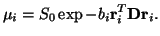
matrix is proportional to the diffusion tensor,  . The
resulting diffusion weighted signal,
. The
resulting diffusion weighted signal,  along a gradient direction
 , with
  -value
  is modeled as:
 |
(5) |
where  is the signal with no diffusion gradients applied. ,
the diffusion tensor is:
is the signal with no diffusion gradients applied. ,
the diffusion tensor is:
![$\displaystyle \vec{D}=\left[ \begin{array}{ccc} D_{xx}&D_{xy}&D_{xz}\\ D_{xy}&D_{yy}&D_{yz}\\ D_{xz}&D_{yz}&D_{zz} \end{array}\right]$](img28.png) |
(6) |
When performing point estimation of the parameters in the diffusion
tensor model, it has been convenient to choose the free parameters in
the model to be the 6 independent elements of the tensor,
 , and the signal strength when no diffusion gradients
are applied,. This parametrization allows estimation to take the
form of a simple least squares fit to the log data. When sampling,
however, our choice of parametrization is far less constrained by our
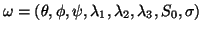
estimation technique. The parameters of real interest in the tensor
are the three eigenvalues, and the three angles defining the shape and
orientation of the tensor. By choosing these as the free
parameters in the model , not only do we give ourselves immediate
access to the posterior pdfs on the parameters of real interest, but
we also allow ourselves the freedom to apply constraints or add
information exactly where we would like to. As a simple example, as
will be seen later, a sensible choice of prior distribution on the
eigenvalues makes it easy to constrain them to be positive. So the
Diffusion Tensor is now parametrized as follows:
, and the signal strength when no diffusion gradients
are applied,. This parametrization allows estimation to take the
form of a simple least squares fit to the log data. When sampling,
however, our choice of parametrization is far less constrained by our
estimation technique. The parameters of real interest in the tensor
are the three eigenvalues, and the three angles defining the shape and
orientation of the tensor. By choosing these as the free
parameters in the model , not only do we give ourselves immediate
access to the posterior pdfs on the parameters of real interest, but
we also allow ourselves the freedom to apply constraints or add
information exactly where we would like to. As a simple example, as
will be seen later, a sensible choice of prior distribution on the
eigenvalues makes it easy to constrain them to be positive. So the
Diffusion Tensor is now parametrized as follows:
 |
(7) |
where
![$\displaystyle \vec{\Lambda}=\left[ \begin{array}{ccc} \lambda_1&0&0\\ 0&\lambda_2&0\\ 0&0&\lambda_3 \end{array} \right]$](img31.png) |
(8) |
and  rotates
 to (
to (
 ), such
that the tensor is first rotated so that its principal eigenvector
aligns with (
), such
that the tensor is first rotated so that its principal eigenvector
aligns with (
 ) in spherical polar coordinates, and then
rotated by
) in spherical polar coordinates, and then
rotated by  around its principal
eigenvector1.
around its principal
eigenvector1.
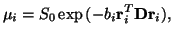
The noise is modeled separately for each voxel as independently
identically distributed (iid) Gaussian. with a mean of zero and
standard deviation across acquisitions of  . The probability
of seeing the data at each voxel
. The probability
of seeing the data at each voxel  given the model,
  , and
any realization of parameter set,
, and
any realization of parameter set,
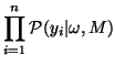
 may now be written as:
where  is the number of acquisitions, and
  and are the
measured and predicted values of the
and are the
measured and predicted values of the
 acquisition
respectively. (Note that throughout this paper,
acquisition
respectively. (Note that throughout this paper,  will be used to
index acquisition number).
will be used to
index acquisition number).
 |
(10) |
Thus, the model at each voxel has 8 free parameters each of which is
subject to a prior distribution. Priors are chosen to be
non-informative, with the exception of ensuring positivity where
sensible2.
Parameters  and in the Gamma distributions are chosen to give
these priors a suitably high variance such that they have little
effect on the posterior distributions except for where we ensure
positivity. Note that the non-informative prior in angle space is
proportional to
and in the Gamma distributions are chosen to give
these priors a suitably high variance such that they have little
effect on the posterior distributions except for where we ensure
positivity. Note that the non-informative prior in angle space is
proportional to
 ensuring that every elemental area on the
surface of the sphere,
ensuring that every elemental area on the
surface of the sphere,
 has the same prior probability.
Subsections
Next: A Simple Partial Volume
Up: Local Parameter Estimation
Previous: Local Parameter Estimation
Tim Behrens
2004-01-22