


Next: Local Parameter Estimation: Methods
Up: Local Parameter Estimation: Theory
Previous: A Simple Partial Volume
Increasing the Complexity - A Distribution of Fibers?
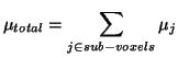
In the partial volume model presented above, only a single fibre
orientation is modeled in each voxel. In fact, there will be a distribution,
 , of fibre orientations in the
voxel. In order to estimate this distribution we must build a model
which, given this distribution, could predict the Diffusion Weighted
MR measurements.
, of fibre orientations in the
voxel. In order to estimate this distribution we must build a model
which, given this distribution, could predict the Diffusion Weighted
MR measurements.
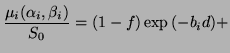
Such a model clearly requires some assumptions. We start by assuming
that each subvoxel has only one fibre direction through it and that
the MR signal is the sum of the signal from arbitrarily small
subvoxels, and that the signal from each subvoxel behaves as
described by Equation 12. (Note that this is a strong
assumption to make, but it is explicit in the model. Any other
model of the local diffusion characteristics of a single fibre
orientation may be used as a replacement.)
 |
(16) |
where
 is the vector of MR signal from the voxel at each
gradient direction and strength, and
is the vector of MR signal from the voxel at each
gradient direction and strength, and
 is the same vector
for each sub-voxel.
is the same vector
for each sub-voxel.
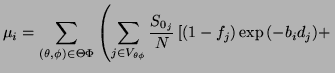
If we now consider, instead of the individual sub-voxels, the set
 of major directions (
 ) in these subvoxels
(note the discretization of
) , then Equation
16 is identically equivalent to (see equation
12):
) in these subvoxels
(note the discretization of
) , then Equation
16 is identically equivalent to (see equation
12):
 |
|
|
|
![$\displaystyle \left.\vphantom{\sum_{(\theta,\phi)\in\Theta\Phi}\left(\sum_{j\in...
...}_i^T\vec{R}_{\theta\phi}\vec{A}\vec{R}_{\theta\phi}^T\vec{r}_i)}\right]\right)$](img83.png) |
|
|
(17) |
where
 is the set of all voxels whose principal fibre
direction is
is the set of all voxels whose principal fibre
direction is
 and
and  is the number of subvoxels. This
equation, although fearsome at first sight, is actually very straight
forward. The first part of the argument to the summation (on the top
line) represents the signal due to all of the isotropic compartments,
and the second part represents the signal due to all of the fibre
compartments. If we now further assume that
is the number of subvoxels. This
equation, although fearsome at first sight, is actually very straight
forward. The first part of the argument to the summation (on the top
line) represents the signal due to all of the isotropic compartments,
and the second part represents the signal due to all of the fibre
compartments. If we now further assume that  (the signal with no
diffusion gradients applied) and
(the signal with no
diffusion gradients applied) and  (the diffusivity) are constant
across the voxel, then the inner summation (over voxels which have
the same principal direction) may be replaced by a constant for the
isotropic compartment, and in the anisotropic compartments, by the
distribution function
defined earlier. With a little
more manipulation and by letting the sub-voxel size tend to zero, it
is easy to arrive at:
(the diffusivity) are constant
across the voxel, then the inner summation (over voxels which have
the same principal direction) may be replaced by a constant for the
isotropic compartment, and in the anisotropic compartments, by the
distribution function
defined earlier. With a little
more manipulation and by letting the sub-voxel size tend to zero, it
is easy to arrive at:
 |
|
|
|
 |
|
|
(18) |
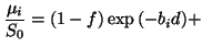
where  is now the proportion of the whole voxel showing isotropic
diffusion.Note that the integral is over
is now the proportion of the whole voxel showing isotropic
diffusion.Note that the integral is over
 in order to
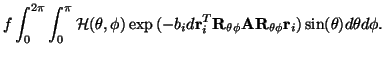
maintain elemental area over the sphere. Finally, if we write the
gradient direction
in order to
maintain elemental area over the sphere. Finally, if we write the
gradient direction  in spherical polar coordinates
![$ \vec{r}_i=[\begin{array}{ccc} \sin{\alpha_i}\cos{\beta_i}&
\sin{\alpha_i}\sin{\beta_i}& \cos{\alpha_i}
\end{array}],$](img90.png) and define
and define  as the angle between gradient direction,
 , and fibre direction
 ,
then the exponent inside the integral reduces dramatically. We may now
write:
,
then the exponent inside the integral reduces dramatically. We may now
write:
 |
|
|
|
![$\displaystyle f\int_0^{2\pi}\int_0^{\pi}\mathcal{H}(\theta,\phi)\exp{}[-b_id\cos^2\gamma_i]\sin(\theta)d\theta
d\phi .$](img95.png) |
|
|
(19) |
This equation reveals a great deal about the diffusion measurement
process. The real ``signal'' of interest is
 , the distribution of fibers within the
voxel. When we measure the diffusion profile of this signal, we are
measuring a version of this signal which is smoothed in angular space,
with a kernel, predicted by this model, of
, the distribution of fibers within the
voxel. When we measure the diffusion profile of this signal, we are
measuring a version of this signal which is smoothed in angular space,
with a kernel, predicted by this model, of
 . We would like to
deconvolve the effect of the measurement process from the signal.
However, we leave the details of this estimation process, and validation
thereof, as future work.
. We would like to
deconvolve the effect of the measurement process from the signal.
However, we leave the details of this estimation process, and validation
thereof, as future work.
Next: Local Parameter Estimation: Methods
Up: Local Parameter Estimation: Theory
Previous: A Simple Partial Volume
Tim Behrens
2004-01-22