In-vivo Human Head

An experimentally acquired field map of an in-vivo human head was used to validate the method in practice. The MR field map sequence used a symmetric-asymmetric spin-echo pair [10,11] (2.5ms asymmetry time; $128 \times 256 \times 20$ voxels of size $1.5 \times 1.0 \times 6.0 mm$). The theoretical field map was calculated using an object susceptibility map that was created from a $112 \times 164 \times 156$ ( $1.0 \times 1.0 \times 1.0 mm$), segmented CT image (as it discriminates between bone and air), which was registered to the MR image corresponding to the acquired field map.

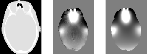
Figure 3 shows slices from the CT image used to define the object susceptibility map, plus both the experimentally acquired field map and the field map calculated using the voxel-based perturbation method described above (execution time was 9 minutes on a 1.8GHz Athlon, 2GB memory running Linux). Note that both field maps have been masked so that only brain tissue is included (although the simulation included all tissues present, with $\chi_\mathrm{brain} = \chi_\mathrm{bone} = 1.0$) and have had the first and second-order spherical harmonics removed in order to factor out the effect of the shims on the field maps.

Qualitatively it can be seen that the match is good. Quantitatively the mean absolute difference between the field maps is 0.05 ppm, while the typical range of the field values (used for the display range in Fig. 3) is $\pm 0.4 ppm$. The calculated error can also be compared with the neglected second order terms in the perturbation expansion. These second order terms have an approximate magnitude of $\delta^2 = 10^{-10} = 0.0001 ppm$, which is two orders of magnitude less than the observed errors. However, there is also another error contribution, from the the inaccuracies in modelling the object as a set of rectangular voxels, which is dominant in this case.

Figure 3: Corresponding slices from images of an in-vivo human head, showing the CT image used to derive the susceptibility map (left), the experimentally acquired field map (middle) and the field map from the voxel-based perturbation calculation (right). The displayed scale of the field maps is $\pm 0.4$ ppm.