Inter-Session Evaluation Methods

For all paradigms and all analysis methods, simple fixed-effects (FE) and OLS mixed-effects (ME) Z-statistics were formed. For each paradigm a mask of voxels which FE considered potentially activated ($Z>2.3$) was created. This contains voxels in which a ME analysis is potentially interested (given that ME generally gives lower Z-statistics than FE⁴). This mask was averaged over A,C,D and E to balance across the various methods, and then eroded slightly (2mm in 3D) to avoid possible problems due to different brain mask effects.

We initially investigated the size of intersession variance, by estimating the ratio of random effects variance to fixed effects, averaged over the voxels of interest as defined above. Given that ME variance is the sum of FE and RE variance, we estimated the RE (intersession) variance by subtracting the FE variance from the ME variance. We then took the ratio image of RE to FE variance, and averaged over the masks described above. This ratio would be 0 if there was no intersession variability and rises as its contribution increases. A ratio of 1 occurs when intersession and intrasession variabilities make similar contributions to the overall measured ME variance.

Next, we investigated whether session variability is indeed Gaussian distributed. If it is not, then inference based on the OLS method used for ME modelling and estimation in this paper would need much more complicated interpretation (as also would be the case with many other group-level methods used in the field). We used the Lilliefors modification of the Kolmogorov-Smirnov test [17] to measure in what fraction of voxels the session effect was significantly non-Gaussian.

The variance ratio figures do not take into account estimated effect size, which in general will vary between methods, and so the primary quantification in this paper uses the mixed-effects Z (ME-Z). This is roughly prortional to the mean effect size and inversely proportional to the intersession variability. This makes ME-Z a good measure with which to evaluate session variability; it is directly affected by the variability, while being weighted higher for voxels of greater interest (i.e., voxels containing activation). We are not particularly interested in variability in voxels which contain no mean effect. We therefore base our cross-subject quantitations on ME-Z comparisons within regions of interest (defined above).⁵

If one of the analysis methods tested here results in increased ME-Z, then this implies reduced overall method-related error (increased accuracy) in the method. This is due to the fact that unrelated variances add; whilst a single-session analysis cannot eliminate true inter-session variance instrinsic to the data, it can add (``induce'') variance to the effective intersession variance due to failings in the method itself (for example, poor estimates of first-level effect/variance, or registration inaccuracies). Therefore the best methods should give ME-variance which approaches (from above) the true, intrinsic inter-session ME-variance. (Remember that the same simple OLS second-level estimation method was used for all analyses carried out - it is only the first-level processing that is varied.)

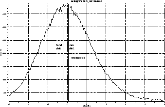
Mean ME-Z was then calculated within the FE-derived masks. However, as well as reporting these ``uncorrected'' mean ME-Z values, we also report the mean values after adjusting the ME-Z images for the fact that in their histograms (supposedly a combination of a null and an activation distribution) the null part, ideally a zero mean and unit standard deviation Gaussian, was often significantly shifted away from having the null peak at zero. This makes Z values incomparable across methods, and needed to be corrected for. The causes of this effect include (spatially) structured noise in the data and in differences in the succcess between the different methods for correcting for temporal smoothness (a problem enhanced potentially for all methods given the unusually low number of time points in the paradigms).

We used two methods to correct ME-Z for null-distribution imperfections, and report results for both methods. With hand-corrected peak shift correction, the peak of the ME-Z distribution was identified by eye and assumed to be the mean of the null disribution; the ME-Z image then had this value subtracted. With mixture-model-based null shift correction, a (non-spatial) histogram mixture model was automatically fitted to the data using expectation-maximisation. This involved a Gaussian for the null part, and gammas for the activation and deactivation parts [2]. The centre of the Gaussian fit was then used to correct the ME-Z image. The advantage of the hand-corrected method is that it is potentially less sensitive to failings in the assumed form of the mixture components; the advantage of the mixture-model-corrected fit is that it is fully automated and therefore more objective.

It is not yet standard practice (with either SPM or FSL) to correct for null-Z shifts in ME-Z histograms; the most common method of inference is to use simple null-hypothesis testing on uncorrected T or Z maps (typically via Gaussian random field theory). By correcting for the shifts, what we are able to investigate the effects of using the different individual analysis components in the absence of confounding effects of null distribution imperfections.

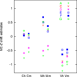
Figure 1 shows an example ME-Z histogram including the estimates (by eye and by mixture-modelling) of the null mode. The estimated ME-Z shifts which were applied to the mean ME-Z values before comparing methods are plotted for all analysis methods and all paradigms in Figure 2. The shift is clearly more related to the choice of time-series statistics method than the choice of spatial processing method (motion correction and registration), but there is no clear indication of one statistics method giving greater shift extent than another. The two correction methods are largely in agreement with each other.

Figure 1: Example ME-Z histogram showing null-distribution shift, from analysis A of the visual paradigm.

Figure 2: Estimated ME-Z null-distribution shifts. Different tasks: C=cognitive M=motor V=visual. Different correction methods: h=hand-shifted m=mixture-model-shifted.