Example Box: Distortion Correction with Fieldmaps

Introduction

The aim of this example is to become familiar with how to use gradient-echo fieldmaps to perform distortion correction and registration of fMRI and structural images.

This example is based on tools available in FSL, and the file names and instructions are specific to FSL. However, similar analyses can be performed using other neuroimaging software packages.

Please download the dataset for this example here:

Data download

The dataset you downloaded contains the following:

Original (non-brain-extracted) T1-weighted image: T1.nii.gz
A single 3D volume from a functional acquisition: func.nii.gz
A fieldmap acquisition (phase and magnitude): fmap_phase.nii.gz and fmap_mag.nii.gz
Directory containing previously generated results: pre_baked

Fieldmap preparation

This section is the same as in the previous example box - if you have already done this then skip ahead to the next section.

The first step is to process the raw fieldmap images to get them into the required form for subsequent registration. This can be done in FSL with the following commands:

bet fmap_mag.nii.gz fmap_mag_brain1.nii.gz

fslmaths fmap_mag_brain1.nii.gz -ero fmap_mag_brain.nii.gz

fsl_prepare_fieldmap SIEMENS fmap_phase.nii.gz fmap_mag_brain.nii.gz fmap_rads.nii.gz 2.46

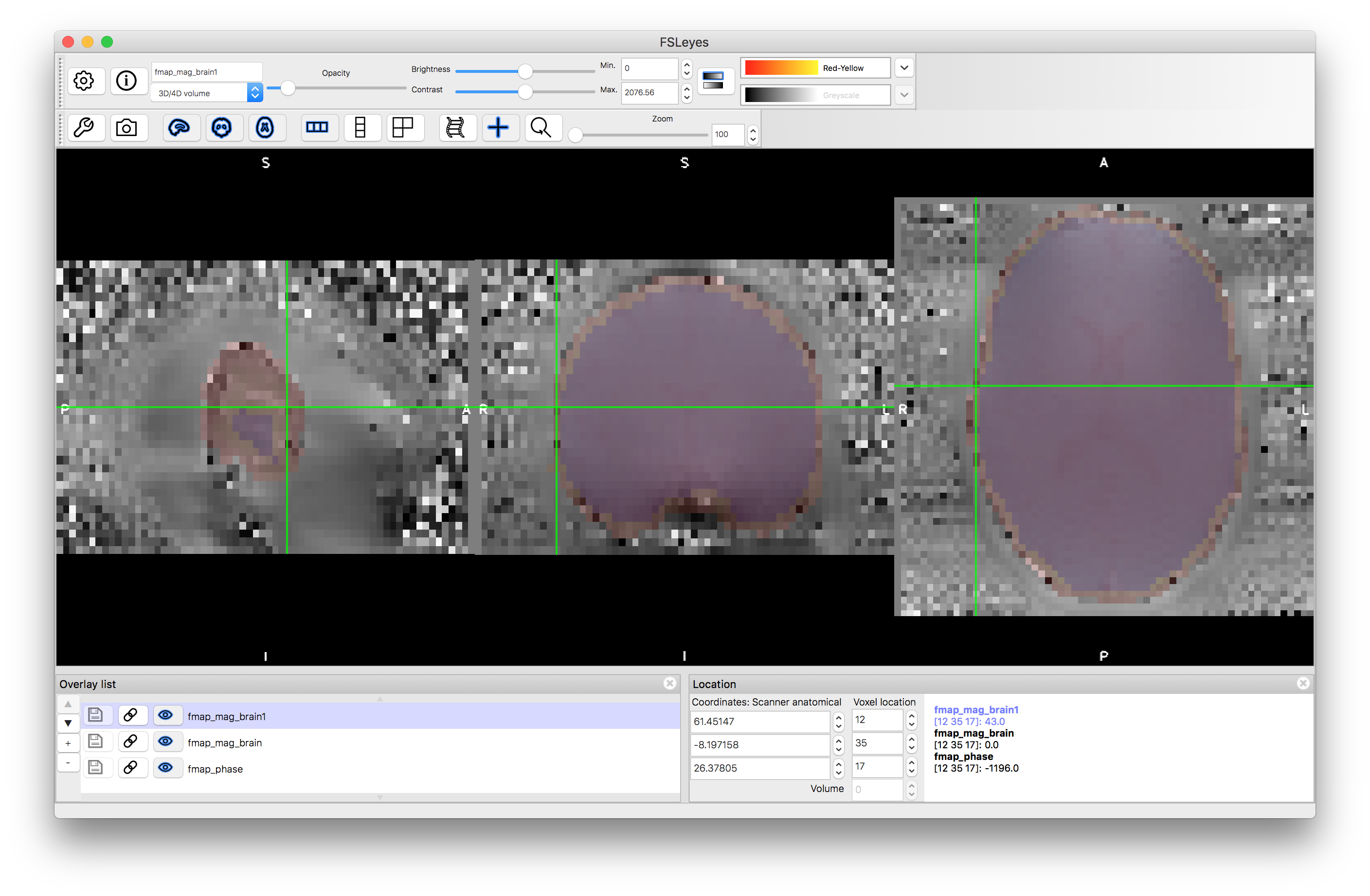
The second step here is necessary to remove noisy edges from phase image but is not necessary in all datasets. Inspect the results of these two brain extraction steps: fmap_mag_brain1.nii.gz and fmap_mag_brain.nii.gz to see the difference, and also load the fmap_phase.nii.gz image to see the noisy values at the edge (e.g. give the two brain extractions different colours, make them quite transparent, and put them on top of the phase image - so that you can see if the brain extractions cover the noisy voxels at the edge or not - see image below).

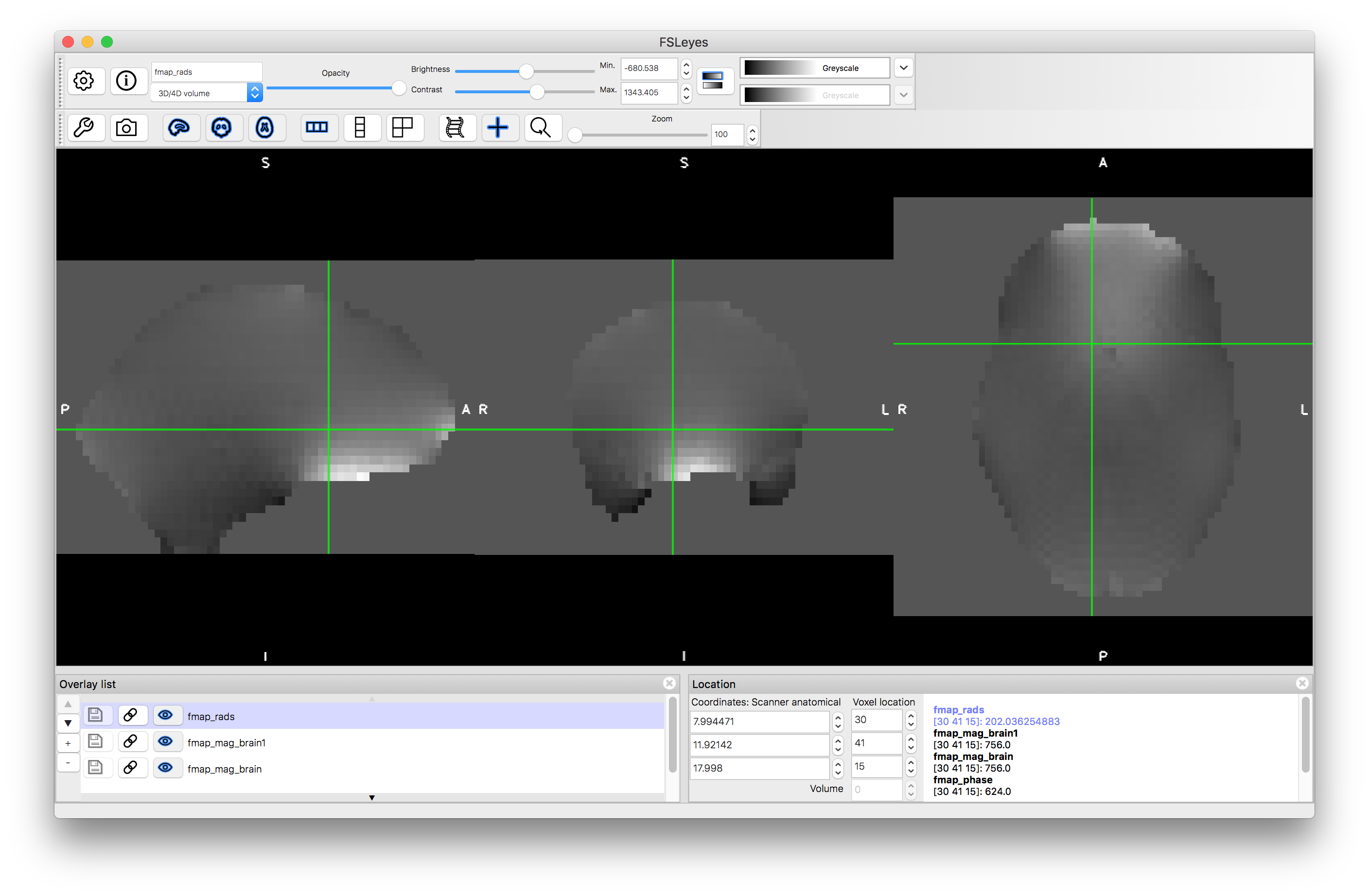
The third command above performs some masking and scaling operations to the phase image, to covert it into the required units of radians per second (denoted by rads in the filename). For this it needs to know one key parameter value, which is the difference in echo times used within the fieldmap acquisition. In this case it was 2.46 milliseconds, but this may vary on different scanners and at different sites, so ask your scanner operator to provide you with this value when you do your own fieldmap scans (if you use the gradient-echo style - see another example box for details on the blip-up-blip-down alternative). View the output fmap_rads - it should look very similar to the phase image, just masked and with the intensities scaled differently.

Structural preparation

It is also necessary to perform brain extraction and segmentation on the T1-weighted structural image. The segmentation is needed by the BBR registration in order to identify the desired boundaries - usually the white matter boundary for this registration problem (fMRI to structural). We will do this with the following commands:

bet T1.nii.gz T1_brain.nii.gz

fast -B -I 10 -l 10 T1_brain.nii.gz

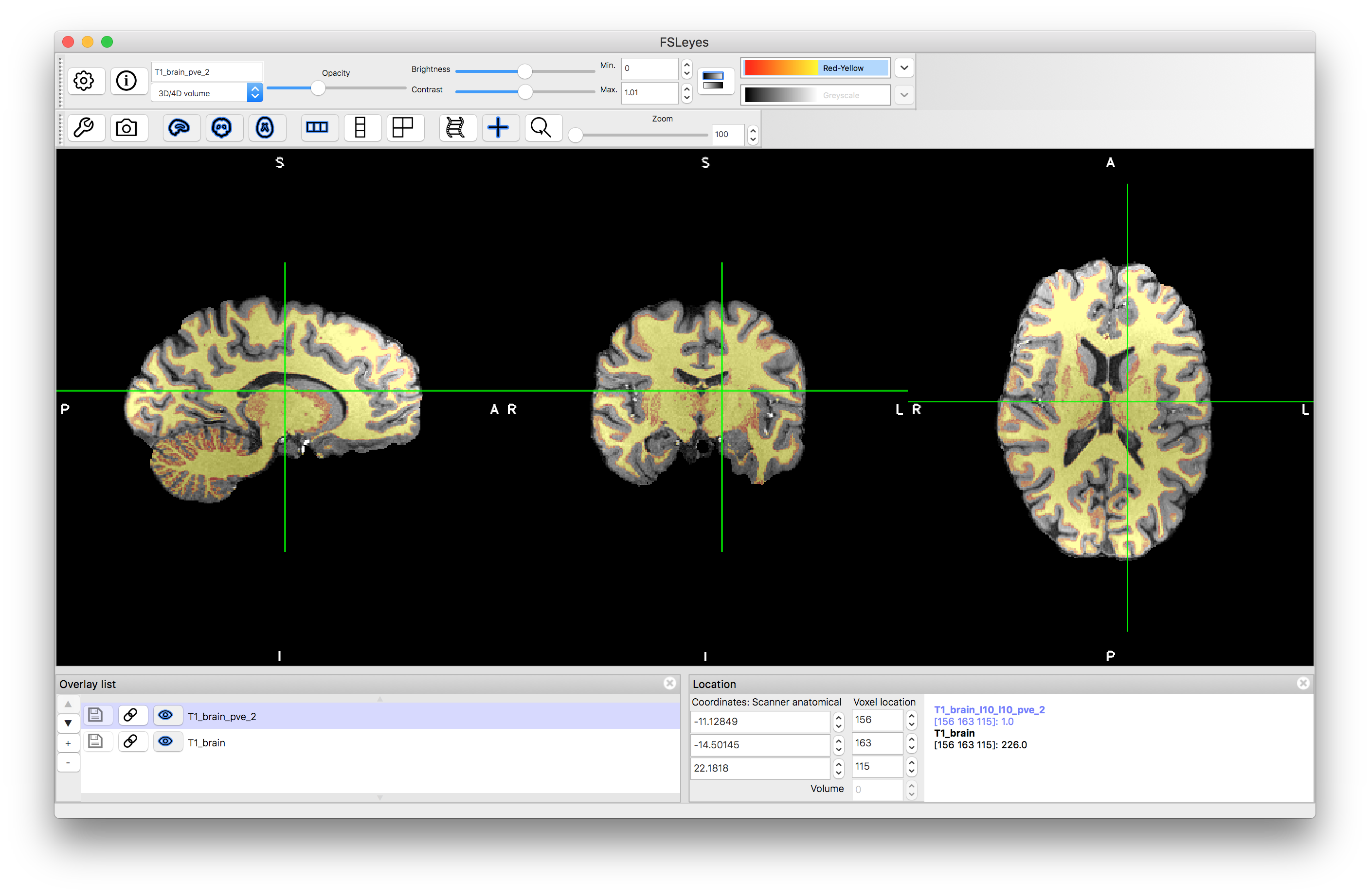
In this case some extra options are used in the call to fast to improve its performance, due to the high resolution and relatively strong bias field. This creates several outputs, of which the most important one for our purposes here is the white matter partial volume estimate: T1_brain_pve_2.nii.gz. Load this, along with the T1_brain.nii.gz to assess the performance (e.g. use the colourmap "Red-Yellow" and look at the voxels in yellow, as those that are orange-red represent small, but non-zero partial volume values). You will find that the segmentation is not perfect, but it identifies the vast majority of the white matter boundary sufficiently accurately for BBR, which just requires finding a global 6 DOF transformation.

From the white matter PVE we then need to make a binary segmentation, which will be used to identify the boundary points. We will treat all voxels with more than 50% partial volume as part of the binary mask, using the following command:

fslmaths T1_brain_pve_2.nii.gz -thr 0.5 -bin T1_wmseg.nii.gz

BBR registration

Now that the fieldmap and the structural image are processed we can apply the BBR registration of the fMRI (EPI) to the structural, using the fieldmap information to correct for geometric distortion.

There are two parameters relating to the EPI (fMRI) sequence that are needed when using fieldmaps. These are:

Effective echo spacing (also known as "dwell time")
- This is the amount of time it takes to acquire individual lines in k-space (the details of what this means are not important). Your scanner operator will be able to provide you will this value. It is typically around 0.3 to 1.0 milliseconds for most modern sequences. If you are using in-plane acceleration (e.g. GRAPPA or SENSE) then the raw echo spacing needs to be divided by the acceleration factor to get the "effective echo spacing".
Phase encoding direction
- This is the voxel coordinate axis of the phase encoding, along which the distortion takes place. It also requires a sign: positive or negative. There are many factors in the scan specification, image reconstruction, format conversion and pre-processing that can change the sign, so it is extremely difficult to determine in advance. Hence the recommended way to determine this in practice is just to try both positive and negative options and see which one gives the better distortion correction - we will do this below. This process only needs to be done once for any study, as the sign will be consistent across the data for all subjects.

For this particular dataset the effective echo spacing is 0.5 milliseconds. Remember that this is a parameter of the EPI sequence (i.e. the fMRI acquisition) and not the fieldmap sequence. The phase encoding direction is along the y-axis, and so we will run both positive and negative y and compare these results.

In FSL there is a specific script used for applying BBR registration (with or without fieldmaps) to EPI images - epi_reg. The specific command for this example, using the negative y-direction, is:

epi_reg --echospacing=0.0005 --wmseg=T1_wmseg.nii.gz --fmap=fmap_rads.nii.gz \
 --fmapmag=fmap_mag.nii.gz --fmapmagbrain=fmap_mag_brain.nii.gz --pedir=-y \
 --epi=func.nii.gz --t1=T1.nii.gz --t1brain=T1_brain.nii.gz --out=func2struct_negy

and using the positive y-direction it is:

epi_reg --echospacing=0.0005 --wmseg=T1_wmseg.nii.gz --fmap=fmap_rads.nii.gz \
 --fmapmag=fmap_mag.nii.gz --fmapmagbrain=fmap_mag_brain.nii.gz --pedir=y \
 --epi=func.nii.gz --t1=T1.nii.gz --t1brain=T1_brain.nii.gz --out=func2struct_posy

The backslashes at the end of end line are just a convenient way to continue the same command over several lines (so keep them in if you are copying and pasting, but if you are typing it out in one line then leave them out). Also, note that the output names do not have .nii.gz after it in this case, as it is used as the prefix for a host of output names.

After you have run the above commands (and they will take a while to run) list the contents of the current directory (use ls in the terminal, or view it in a graphical file browser) to see the outputs that are created (they will start with the specified prefix func2struct_negy or func2struct_posy). The main outputs of interest are (for the negy version as an example):

func2struct_negy.nii.gz
- the functional image resampled into structural space
func2struct_negy.mat
- spatial transformation from undistorted functional space to structural space (this is a 6 DOF transform)
func2struct_negy_warp.nii.gz
- spatial transformation from distorted functional space to structural space (this is a nonlinear transformation as it includes the nonlinear distortion correction plus the 6 DOF transform between spaces)
func2struct_negy_fast_wmedge.nii.gz
- binary image representing the white matter boundaries from the T1-weighted structural image, which is very useful for viewing and assessing registration quality (normally shown in red on top of transformed functional image)

Load the two main outputs func2struct_negy.nii.gz and func2struct_posy.nii.gz into a viewer as well as the func2struct_negy_fast_wmedge.nii.gz (which is the same for the positive and negative versions) and give this a Red colourmap and put it on top of the Overlay List. Turn on and off the resampled functional images and determine which one is better.

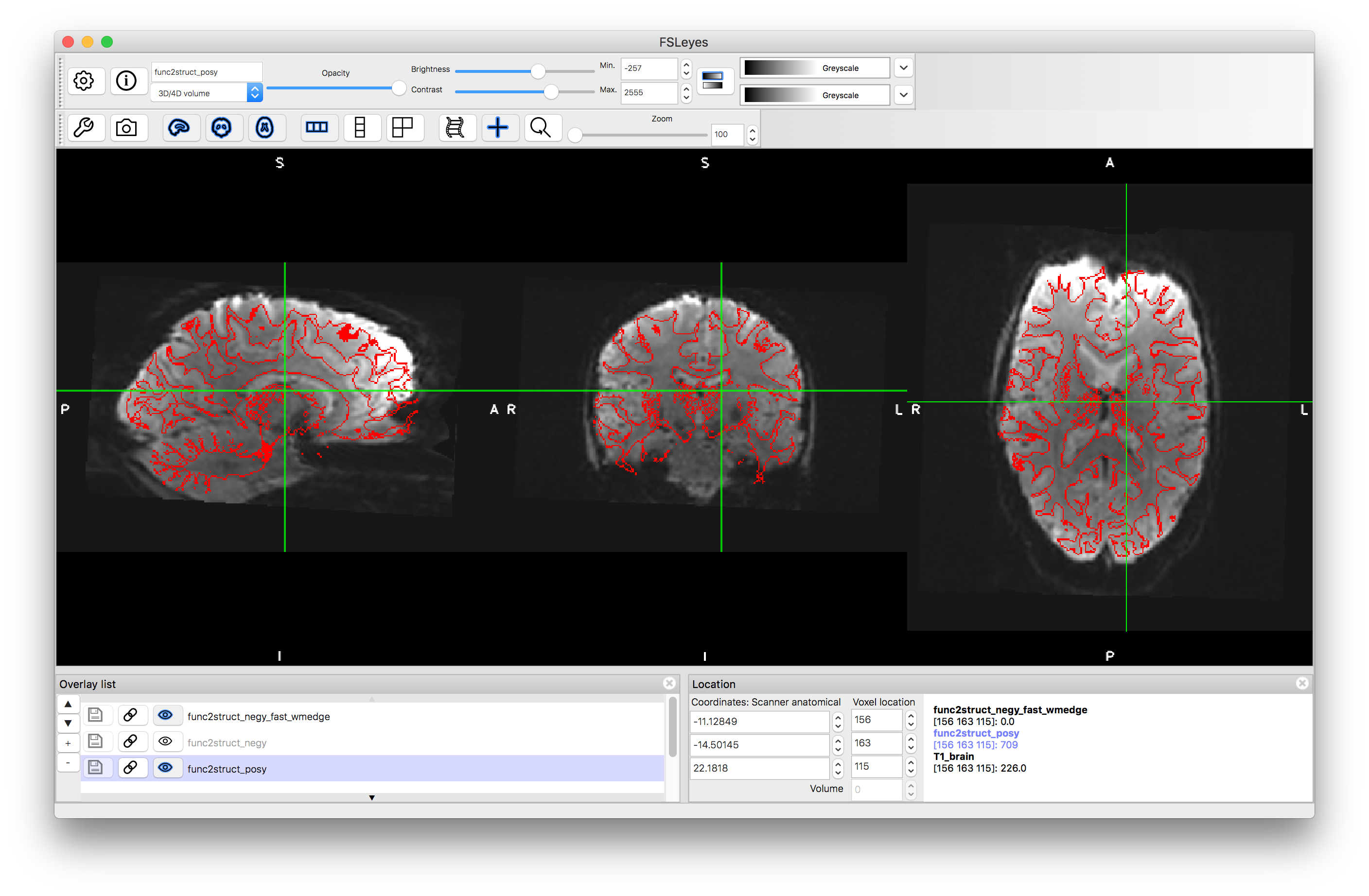
Distortion correction with positive y phase encoding

Distortion correction with negative y phase encoding

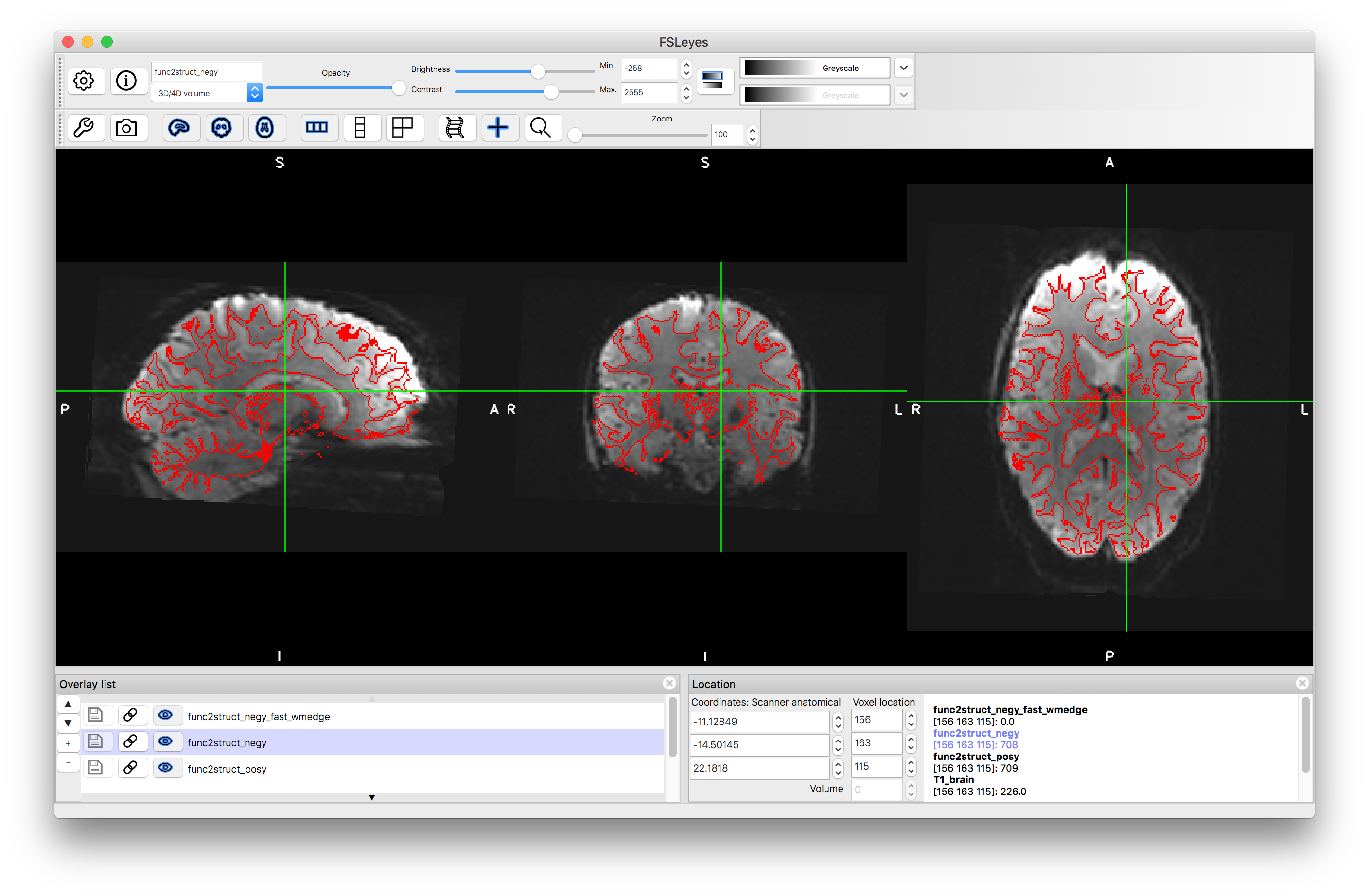
Flicking between the two resampled functional images can be a very good way of seeing the areas where there are substantial changes, corresponding to areas of distortion. It is in these areas that you should concentrate on how well they align with the red boundaries extracted from the structural image. This should help you decide which one has the better alignment. However, do not use areas where there is substantial signal loss to decide on the quality of the alignment, because you cannot distinguish artificial boundaries caused by signal loss from real anatomical boundaries. If you are still unsure which one is better, look at Figure 6.6 in the Primer or click here.

From these examples you should be able to prepare and run a fieldmap-based registration and distortion correction procedure and evaluate the results. This is not the only way to perform distortion correction, but is the recommended way in FSL when using gradient-echo fieldmaps. The alternative to gradient-echo fieldmaps is to use blip-up-blip-down images, which is covered in the next example box.