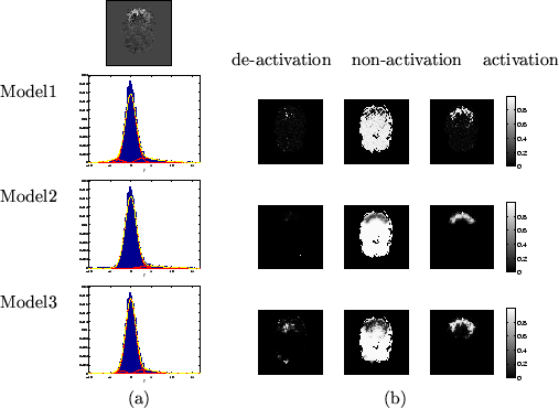
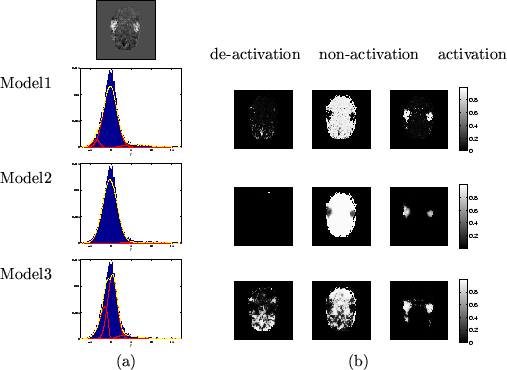
Figures 9 and 10 show the
results of inferring on the three different continuous weights
mixture models we have described on the visual paradigm
and audio paradigm SPMs respectively. The spatial
maps in the figures are unthresholded marginal posterior means
of ![]() , i.e.
, i.e.
![]() for all three classes
of deactivation, non-activation and activation.
Interestingly, the audio dataset shows a large amount of
deactivation. If we qualitatively consider the data
for all three classes
of deactivation, non-activation and activation.
Interestingly, the audio dataset shows a large amount of
deactivation. If we qualitatively consider the data ![]() shown in
the top left of figure 10 then the spatial
pattern of deactivation would seem to be strongly supported.
Model 2, with the spatial smoothness parameter set to
shown in
the top left of figure 10 then the spatial
pattern of deactivation would seem to be strongly supported.
Model 2, with the spatial smoothness parameter set to
![]() imposes too much spatial smoothness. Indeed, if we look at the
adaptively determined spatial smoothness in the
box plot of figure 8, then the
MRF smoothness parameter,
imposes too much spatial smoothness. Indeed, if we look at the
adaptively determined spatial smoothness in the
box plot of figure 8, then the
MRF smoothness parameter,
![]() , for the visual and
audio datasets is far less than the fixed value of
, for the visual and
audio datasets is far less than the fixed value of
![]() used for model 2.
used for model 2.
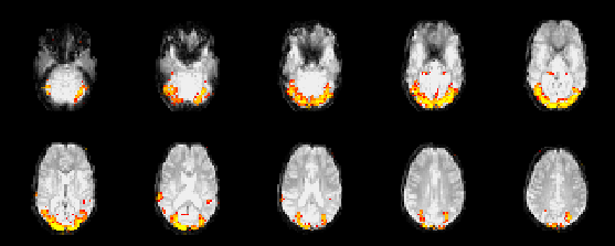
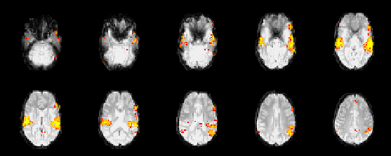
Figures 11 and 12
show maps of the weights for the activation class,
![]() , thresholded to leave only
those voxels with
, thresholded to leave only
those voxels with
![]() for the visual paradigm
and audio paradigm SPMs respectively. The choice of threshold on
for the visual paradigm
and audio paradigm SPMs respectively. The choice of threshold on
![]() is, as with any thresholding, a decision that needs
to be made by the experimenter. However, this is the only
time that any value in the inference of the model has to be chosen.
Indeed, even when we choose the threshold
for
is, as with any thresholding, a decision that needs
to be made by the experimenter. However, this is the only
time that any value in the inference of the model has to be chosen.
Indeed, even when we choose the threshold
for
![]() , there is a natural choice to make. That is we
can choose the threshold of
, there is a natural choice to make. That is we
can choose the threshold of ![]() which gives us an equal
loss function where the chance of a false positive is equal to
the chance of a false negative.
which gives us an equal
loss function where the chance of a false positive is equal to
the chance of a false negative.
 |
 |
 |
 |