Autocorrelation Estimation

An estimate of the autocorrelation matrix $\mathbf{SVS^T}$ of the error $\mathbf{\eta}$ is required. We could estimate $\mathbf{B}$ using equation 2 to obtain the residuals $\mathbf{r}$ and then estimate the autocorrelation matrix of the residuals. However, it can be shown that:

$$\mathbf{r} = \mathbf{RSY} = \mathbf{R\eta}$$ (9)

and then it follows that the autocovariance of the residuals is given by:

$$Cov\{\mathbf{r}\} = \mathbf{\sigma^2RSVS^TR^T}$$ (10)

which is not $\mathbf{SVS^T}$. The difference between the autocorrelation of the error and the autocorrelation of the residuals is clearly due to regression onto the design matrix and it is impossible to unravel $\mathbf{SVS^T}$ from $\mathbf{RSVS^TR^T}$ since $\mathbf{R}$ is noninvertible. This turns out to be not too much of a problem, as can be illustrated using an example time series generated artificially using the noise process $N(0, \sigma _t V_t)$, where $V_t$ is the autocorrelation matrix for the typical grey matter autocorrelation in figure 5(a). Figure 1(a) shows the spectral density of the time series, figure 1(b) shows the spectral density of the residuals $\mathbf{r}$ for the same time series after regression onto the HRF convolved boxcar (shown in figure 7), and figure 1(c) shows the same after regression onto the randomised ISI design (shown in figure 10). Despite some subtle differences in the raw spectral density estimates the Tukey estimates are remarkably similar. This is perhaps surprising, particularly for the randomised ISI design, which covers a large frequency range (see figure10(b)). The primary reason for this is that the spectral density will only be affected at the frequency and phase of the regressors. Secondly, when the regressor has high power at a particular frequency but not at its neighbouring frequencies (this is less true for the randomised ISI design but still has some effect), then spectral density estimation techniques which heavily smooth the spectral density will help rectify this problem further. All techniques considered in this paper do effectively smooth the spectral density.

Figure 1: (a) Shows the spectral density of an artificially generated time series using the noise process $N(0, \sigma _t V_t)$, (b) and (c) show the spectral densities of the residuals $\mathbf{r}$ for the same time series after regression onto the HRF convolved boxcar shown in figure 7 and the randomised ISI shown in figure 10 respectively. Raw spectral density estimates are shown by the solid line and estimation using Tukey windowing (with $M=15$) are shown by the broken line. There is no visible difference between the Tukey estimated spectral densities.

For variance correction or colouring, an estimate of $\mathbf{SVS^T}$ can be calculated from the residuals after equation 2 is used to obtain the parameter estimates. This estimate of $\mathbf{SVS^T}$ is used in equation 3 to give the variance of the parameter estimates.

However, prewhitening requires an estimate of $\mathbf{SVS^T}$ before the BLUE can be computed and equation 3 used. To get round this an iterative procedure is used (Bullmore et al., 1996). Firstly, we obtain the residuals $\mathbf{r}$ using a GLM with $\mathbf{S=I}$. The autocorrelation $\mathbf{V}$ is then estimated for these residuals. Given an estimate of $\mathbf{V}$, $\mathbf{V^{-1}}$ and hence $\mathbf{K^{-1}}$ can be obtained by inverting in the spectral domain (some autocorrelation models, e.g. autoregressive, have simple parametrised forms for $\mathbf{K^{-1}}$, and hence inversion in the spectral domain is not necessary). Next, we use a second linear model with $\mathbf{S=K^{-1}}$, and the process can then be repeated to obtain new residuals from which $\mathbf{V}$ can be re-estimated and so on. We use just one iteration and find that it performs sufficiently well in practice. Further iterations either give no further benefit or cause over-fitting, depending upon the autocorrelation estimation technique used. Autoregressive model fitting procedures which determine the order would do the former, nonparametric approaches(Tukey, multitapering etc.) the latter.

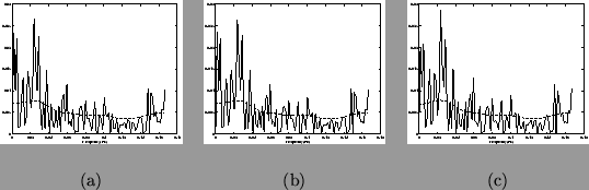
Whether for use in prewhitening, or for correcting the variance and degrees of freedom of the test statistic, an accurate, robust estimate of the autocorrelation is necessary. This estimation could be carried out in either the spectral or temporal domain - they are interchangeable. Raw estimates (equation 11) can not be used since they are very noisy and introduce an unacceptably large bias. Hence some means of improving the estimate is required.

All approaches considered assume second-order stationarity - an assumption whose validity is helped by the use of the non-linear high pass filtering mentioned in the previous section. We consider standard windowing or tapering spectral analysis approaches, multitapering, parametric ARMA and a nonparametric technique which uses some simple constraints. The results of these different techniques applied to a typical grey-matter voxel in a rest/null data are shown for comparison in figure 2.