Introduction

Data analysis often has to proceed on measurements which are intricate mixtures of the initial signal sources of interest. Unless accurate information is available to allow for informed estimation, this is a challenging problem. A possible solution is to employ what is known in the area of signal processing as blind source separation (BSS) techniques [Jutten and Herault, 1991].

The signal of functional magnetic resonance imaging studies is a prime example, comprising different sources of variability, possibly including machine artefacts, physiological pulsation, head motion and haemodynamic changes induced by different experimental conditions. This mixture of signals presents a huge challenge for analytical methods attempting to identify stimulus- or task-related changes.

The vast majority of analytical techniques currently applied to FMRI data test specific hypotheses about the expected BOLD response at the individual voxel locations using simple regression or more sophisticated models like the General Linear Model¹ (GLM) [Worsley and Friston, 1995]. There, the expected signal changes are specified as regressors of interest in a multiple linear regression framework and the estimated regression coefficients are tested against a null hypothesis that these values are distributed according to some known null distribution. These voxel-wise test statistics form summary images known as statistical parametric maps which are commonly assessed for statistical significance using voxel-wise null-hypothesis testing or testing for the size or mass of suprathresholded clusters [Poline et al., 1997]. These approaches are confirmatory in nature and make strong prior assumptions about the spatio-temporal characteristics of signals contained in the data. Naturally, the inferred spatial patterns of activation depend on the validity and accuracy of these assumptions. The most obvious problem with hypothesis-based techniques is the possible presence of unmodelled artefactual signal in the data. Structured noise which is temporally non-orthogonal to an assumed regression model will bias the parameter estimates, and noise orthogonal to the design will inflate the residual error, thus reducing statistical significance. Either way, any discrepancy between the assumed and the 'true' signal space will render the analysis sub-optimal. Furthermore, while there is a growing number of models that explicitly include prior spatial information [Hartvig and Jensen, 2000], the standard GLM approach is univariate and essentially discards information about the spatial properties of the data, only inducing spatial smoothness by convolving the individual volumes with a Gaussian smoothing kernel, and returning to spatial considerations only after modelling has completed (e.g. Gaussian Random Field Theory-based inference [Poline et al., 1997]).

Figure 1: GLM and classical ICA analysis of visual stimulus FMRI data: (i) GLM results using GRF-based inference ( $Z>2.3,p<0.01$); (ii)-(v) IC maps where the correlation of the extracted time course with the expected BOLD response exceeds $0.3$. Both for GLM analysis and ICA, the data was high-pass filtered (Gaussian-weighted local straight line fitting with cutoff of 90s [Marchini and Ripley, 2000]) and spatially smoothed with a Gaussian kernel of 3mm (FWHM). ICA maps were thresholded at $Z>2.3$ after transformation into "$Z$-scores" across the spatial domain as described in [McKeown et al., 1998]. Note that this should not be confused with GLM or PICA $Z$-score thresholding as described in section 4, where $Z$-scores are formed by dividing by the voxel-wise estimated standard deviation of the noise.

As one alternative to hypothesis-driven analytical techniques, Independent Component Analysis (ICA, [Comon, 1994]) has been applied to FMRI data as an exploratory data analysis technique in order to find independently distributed spatial patterns that depict source processes in the data [McKeown et al., 1998,Beckmann et al., 2000]. The basic goal of ICA is to solve the BSS problem by expressing a set of random variables (observations) as linear combinations of statistically independent latent component variables (source signals).

There have been primarily two different research communities involved in the development of ICA. Firstly, the study of mixed sources is a classical signal processing problem. The seminal work into BSS [Jutten and Herault, 1991] looked at extensions to standard principal component analysis (PCA). Theoretical work on high order moments provided one of the first solutions to a BSS problem [Cardoso, 1989]. [Jutten and Herault, 1991] published a concise presentation of their adaptive algorithm and outlined the transition from PCA to ICA very clearly. Their approach has been further developed by [Karhunen and Joutsensalo, 1995] and [Cichocki et al., 1994]. Exact conditions for the identifiability of the model can be found in [Comon, 1994] together with an algorithm that approximates source signal distributions using their first few moments, a technique that was also employed by other authors [Deco and Obradovic, 1995].

In parallel to blind source separation studies, unsupervised learning rules based on information theoretic principles were proposed by [Linsker, 1988]. These learning rules are based on the principle of redundancy reduction as a coding strategy for neurons of the perceptual system [Attneave, 1954].

More recently, [Baram and Roth, 1994] and [Bell and Sejnowski, 1995] introduced a surprisingly simple blind source separation algorithm for a non-linear feed-forward network from an information maximization viewpoint. This algorithm was subsequently improved, extended and modified [Amari, 1997] and its relation to maximum likelihood estimation and redundancy reduction was investigated [MacKay, 1996]. There now exists a variety of alternative algorithms and principled extensions that include work on non-linear mixing, non-instantaneous mixing, incorporation of source structure and observational noise.

Classical Independent Component Analysis has been popularised in the field of FMRI analysis by [McKeown et al., 1998], where the data from the FMRI experiment with $n$ voxels measured at $p$ different time points is written as a $p\times n$ matrix $X$ for which a decomposition is sought such that

$$\mbox{\protect\boldmath$X$} = \mbox{\protect\boldmath$A$} \mbox{\protect\boldmath$S$} .$$ (1)

The matrix $S$ is optimized to contain statistically independent spatial maps in its rows, i.e. spatial areas in the brain, each with an internally consistent temporal dynamic, which is characterised by a time-course contained in the associated column of the square mixing matrix $A$. In [McKeown et al., 1998], the sources are estimated by iteratively optimising an unmixing matrix $W$$=$$A$$^{-1}$ so that $S$$=$$W$$X$ contains mutually independent rows, using the infomax algorithm [Bell and Sejnowski, 1995].

The ICA model above, though being a simple linear regression model, differs from the standard GLM as used in neuroimaging in two essential aspects: firstly, the mixing is assumed to be square, i.e. the signal is not constrained to be contained within a lower dimensional signal sub-space. Secondly, the model of equation 1 does not include a noise model. Instead, the data are assumed to be completely characterized by the estimated sources and the mixing matrix. This, in turn, precludes the assessment of statistical significance of the source estimates within the framework of null-hypotheses testing. Both problems are strongly linked in that if we relax the assumption on square mixing by requesting a smaller number of source processes to represent the dynamics in the data, we automatically introduce a mismatch between the best linear model fit and the original data. In analogy to the GLM case, the residual error will be the difference between what the model can explain and what we actually observe.

In the absence of a suitable noise model, slightest differences in the measured hæmodynamic response at two different voxel locations are necessarily treated as 'real effects'. These differences might represent valid spatial variations, e.g. slightly different temporal responses between left and right hemisphere or simply differences in the background noise level (e.g. spatial variations due to the image acquisition, sampling etc.), and may cause clusters of voxels that 'activate' to the same external stimulus to be fragmented into different spatial maps - a split into what in [McKeown et al., 1998] has been termed consistently and transiently task related components occurs. The noise free generative model precludes any test for significance and threshold techniques like converting the component map values into $Z$-scores [McKeown et al., 1998] are devoid of statistical meaning and can only be understood as ad-hoc recipes (see section 4).

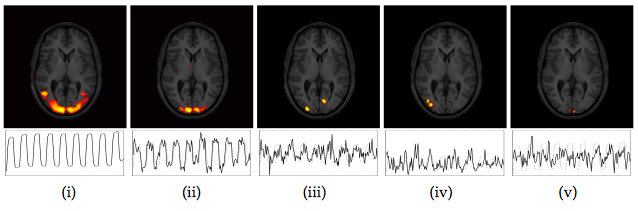
As an example, figure 1 shows the results of a GLM analysis of a simple FMRI data set from a visual stimulation experiment (30s on/off block design with a black/white checkerboard reversing at 8Hz during the on condition).

Though visual experiments of this kind are generally expected to generate consistent activation maps over a wide range of analysis techniques, the spatial maps of GLM analysis and ICA differ substantially. While one of the ICA maps clearly depicts activation in the primary visual areas (ii), the spatial extent differs from areas found using a GLM analysis (i). This is only partly due to the arbitrary IC map thresholding; the lateral anterior activation foci in the GLM map cannot be obtained within the IC map without dramatically inflating the number of voxels classified as active. In addition to the one highly correlated IC map, three additional component maps have an associated time course which correlates with the experimental paradigm² at $r>0.3$. Their spatial activation patterns, though being well clustered and localised inside visual cortical areas, do not lend themselves to easy interpretation.

This is the classical problem of over-fitting a noise-free generative model to noisy observations [Bishop, 1995] and needs to be resolved by setting up a suitable probabilistic model that controls the balance between what is attributable to 'real effects' of interest and what simply is due to observational noise.

In order to address these issues we examine the probabilistic Independent Component Analysis (PICA) model [Penny et al., 2001,Beckmann et al., 2001] for FMRI data that allows for a non-square mixing process and assumes that the data are confounded by additive Gaussian noise.

In the case of isotropic noise covariance the task of blind source separation can be divided into three stages: (i) estimation of a signal + noise sub-space that contains the source processes and a noise sub-space orthogonal to the first, (ii) estimation of independent components in the signal + noise sub-space and (iii) assessing the statistical significance of estimated sources.

At the first stage we employ probabilistic Principal Component Analysis (PPCA, [Tipping and Bishop, 1999]) in order to find an appropriate linear sub-space which contains the sources. The choice of the number of components to extract is a problem of model order selection. Underestimation of the dimensionality will discard valuable information and result in suboptimal signal extraction. Overestimation, however, results in a large number of spurious components due to underconstrained estimation and a factorization that will overfit the data, harming later inference and dramatically increasing computational costs.

Within the probabilistic PCA framework we will demonstrate that the number of source processes can be inferred from the covariance matrix of the observations using a Bayesian framework that approximates the posterior distribution of the model order [Minka, 2000] and extending this approach to take account of the limited amount of data and the particular structure of FMRI noise [Beckmann et al., 2001].

At the second stage the source signals are estimated within the lower- dimensional signal + noise sub-space using a fixed-point iteration scheme [Hyvärinen et al., 2001] that maximises the non-Gaussianity of the source estimates. Finally, at the third level, the extracted spatial maps are converted into '$Z$ statistic' maps based on the estimated standard error of the residual noise. These maps are assessed for significantly modulated voxels using a Gaussian Mixture Model for the distribution of intensity values.

The paper is organised as follows. Section 2 defines the probabilistic ICA model and discusses the uniqueness of the solution. Estimation of the model order, the mixing process and the sources is outlined in section 3. Section 4 discusses the Gaussian Mixture Model approach to IC map thresholding. Finally, sections 5 and 6 demonstrate the technique on artificial and real FMRI data and some discussion and concluding comments are given in sections 7 and 8.