The maximum likelihood solutions given in equations
5-7 depend on knowledge of the latent dimensionality ![]() . In the noise free case this quantity can
easily be deduced from the rank of the covariance of the observations
. In the noise free case this quantity can
easily be deduced from the rank of the covariance of the observations
Many other informal methods have been
proposed, the most popular choice being the "scree plot" where one
looks for a "knee" in the plot of ordered eigenvalues that signifies a
split between significant and presumably unimportant directions of the
data. With real FMRI data, however, the decision as to where to choose the
cutoff value is not obvious and a choice based on simple visual
inspection will be ambiguous (see figure 9(ii) for an example).
This problem is intensified by the fact
that the data set
![]() is finite and thus
is finite and thus
![]()
![]() is being estimated by the
sample covariance of the set of observations
is being estimated by the
sample covariance of the set of observations
![]() . Even in the absence of any source signals, i.e. when
. Even in the absence of any source signals, i.e. when
![]() contains a
finite number of samples from purely Gaussian isotropic noise only, the
eigenspectrum of the sample covariance matrix is not identical to
contains a
finite number of samples from purely Gaussian isotropic noise only, the
eigenspectrum of the sample covariance matrix is not identical to ![]() but
instead distributed around the true noise covariance: the eigenspectrum will
depict an apparent difference in the significance of individual directions
within the noise [Everson and Roberts, 2000].
but
instead distributed around the true noise covariance: the eigenspectrum will
depict an apparent difference in the significance of individual directions
within the noise [Everson and Roberts, 2000].
|
In the case of purely Gaussian noise, however, the sample covariance matrix
![]() has a Wishart distribution and we can utilise
results from random matrix theory on the empirical
distribution function
has a Wishart distribution and we can utilise
results from random matrix theory on the empirical
distribution function ![]() for the eigenvalues of the covariance matrix of
a single random
for the eigenvalues of the covariance matrix of
a single random ![]() -dimensional matrix
-dimensional matrix
![]() [Johnstone, 2000].
Suppose that
[Johnstone, 2000].
Suppose that
![]() as
as
![]() and
and
![]() , then
, then
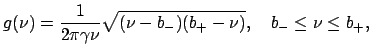
![]() almost surely, where the limiting distribution has a density
almost surely, where the limiting distribution has a density
If we assume that the source distributions
![]()
![]()
![]() are Gaussian, the
probabilistic ICA model (equation 2) reduces to the
probabilistic PCA model [Tipping and Bishop, 1999]. In this case, we can use more
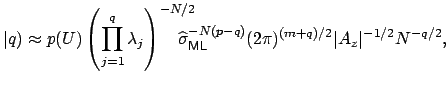
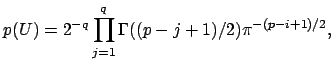
sophisticated statistical criteria for model order selection. [Minka, 2000]
placed PPCA in the Bayesian framework and presented a Laplace approximation to
the posterior distribution of the model evidence that
can be calculated
efficiently from the eigenspectrum of the covariance matrix of
observations. When
are Gaussian, the
probabilistic ICA model (equation 2) reduces to the
probabilistic PCA model [Tipping and Bishop, 1999]. In this case, we can use more
sophisticated statistical criteria for model order selection. [Minka, 2000]
placed PPCA in the Bayesian framework and presented a Laplace approximation to
the posterior distribution of the model evidence that
can be calculated
efficiently from the eigenspectrum of the covariance matrix of
observations. When
![]() min
min![]() , then
, then
In order to account for the limited amount of data, we combine this estimate
with the predicted cumulative distribution and replace
![]() by its
adjusted eigenspectrum
by its
adjusted eigenspectrum
![]()
![]() prior to evaluating the
model evidence. Other possible choices for model order selection for PPCA
include the Bayesian Information Criterion (BIC, [Kass and Raftery, 1993]) the
Akaike Information Criterion (AIC, [Akaike, 1969]) or Minimum
Description Length (MDL, [Rissanen, 1978]).
prior to evaluating the
model evidence. Other possible choices for model order selection for PPCA
include the Bayesian Information Criterion (BIC, [Kass and Raftery, 1993]) the
Akaike Information Criterion (AIC, [Akaike, 1969]) or Minimum
Description Length (MDL, [Rissanen, 1978]).
Note that the estimation of the model order in the case of the
probabilistic PCA model is based on the assumption of Gaussian source
distribution. [Minka, 2000], however, provides some empirical
evidence that the Laplace approximation works reasonably well in the
case where the source distributions are non-Gaussian.
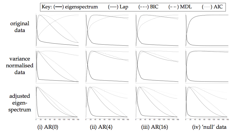
As an example, figure 2 shows the eigenspectrum and different estimators of the intrinsic dimensionality for
different artificial data sets, where 10 latent sources with non-Gaussian distribution were introduced into
simulated AR data (i.e. auto-regressive noise where the AR parameters were
estimated from real resting state FMRI data) and real FMRI resting state noise
at peak levels of between ![]() and
and ![]() of the mean signal intensity. Note
how the increase in AR order will increase the estimates of the latent
dimensionality, simply because there are more eigenvalues that fail the
sphericity assumption. Performing variance-normalisation and adjusting the
eigenspectrum using
of the mean signal intensity. Note
how the increase in AR order will increase the estimates of the latent
dimensionality, simply because there are more eigenvalues that fail the
sphericity assumption. Performing variance-normalisation and adjusting the
eigenspectrum using
![]() in all cases improves the estimation. In the
case of Gaussian white noise the model assumptions are correct and the adjusted
eigenspectrum exactly matches equation 8. In most cases, the
different estimators give similar results once the data were variance
normalised
and the eigenspectrum was adjusted using
in all cases improves the estimation. In the
case of Gaussian white noise the model assumptions are correct and the adjusted
eigenspectrum exactly matches equation 8. In most cases, the
different estimators give similar results once the data were variance
normalised
and the eigenspectrum was adjusted using
![]() . Overall, the Laplace
approximation and the Bayesian Information Criterion appear to give
consistent estimates of the latent dimensionality even though the distribution of the embedded sources are non-Gaussian.
. Overall, the Laplace
approximation and the Bayesian Information Criterion appear to give
consistent estimates of the latent dimensionality even though the distribution of the embedded sources are non-Gaussian.