


Next: Supplementary points
Up: tr00dl2
Previous: Preprocessing before a PTA-modes
Analysing a summary statistic of subjects changes obviously the data analysed, and clearly it
means that this summary ``sufficiently" informs on the distributions. Analysing means, medians or
trimeans can be also a solution to subjects outliers which put into question the choice of the
location parameter. Looking at only one location parameter implicitly suppose the distributions to
be unimodal, which was a sensible assumption here but PTA- modes could be done with a mode
representing different location parameters of the empirical subject distributions. This has not
been done here as we focused on comparing different main location parameters using a PTA-
modes could be done with a mode
representing different location parameters of the empirical subject distributions. This has not
been done here as we focused on comparing different main location parameters using a PTA- modes.
Figure 5:
PTA-modes dose means, medians or
trimeans (data subject scaled) for all bands (absolute energy) for verum versus
placebo versus first baseline : 1 Principal Tensors.
|
|
On fig.5 the first Principal Tensor of the different PTA-modes on means,
medians or trimeans over the 12 subjects for each dose , band, time, and electrode,
as a tensor of order three, is shown. Each analysis constitutes a dose profile analysis,
each left plot of figure fig.5 representing a dose-effect curve (versus time)
for the corresponding principal tensor of the given profile summary. For the 1 mode (
dose  time) a major difference between these three summaries can be seen for the
30mg curve in comparison to the other doses: no apparent dose effect (around peak) is
observed with the mean). The median and trimean give similar results, the
10mg curve becomes flatter for trimean. For the 2
time) a major difference between these three summaries can be seen for the
30mg curve in comparison to the other doses: no apparent dose effect (around peak) is
observed with the mean). The median and trimean give similar results, the
10mg curve becomes flatter for trimean. For the 2 mode (electrode) a
slight gradient towards the back is seen for median and trimean but the three plots
are very similar. The 3
mode (electrode) a
slight gradient towards the back is seen for median and trimean but the three plots
are very similar. The 3 mode (band) representation for mean differs from the
two others mainly on
mode (band) representation for mean differs from the
two others mainly on  ,
,  and
and  .
With small samples the trimean (
.
With small samples the trimean (
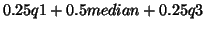 ) seems to be a good compromise
between the two extremes of mean and median either too sensible to outliers or not all. It has
been already used in pharmaco-EEG studies for example by [8]. Analysing means
of the subjects is in fact equivalent to performing a PTAIV-modes on the three-ways arranged
data (i.e. tensor of order three)
) seems to be a good compromise
between the two extremes of mean and median either too sensible to outliers or not all. It has
been already used in pharmaco-EEG studies for example by [8]. Analysing means
of the subjects is in fact equivalent to performing a PTAIV-modes on the three-ways arranged
data (i.e. tensor of order three)  with the following modes :
 as the first mode,
  as the second mode, and
  as the third mode.
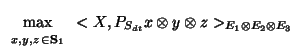
PTAIV means Principal Tensor Analysis with Instrumental Variables and refers to an extension of
PCAIV, [18] or [19], to multiway data, [10]. In the
optimisation procedure one considers linear constraints on the solution defined by the
Instrumental Variables which are usually linked to the design. In our context the optimisation
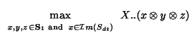
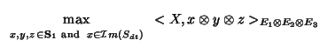
becomes to maximise
as the third mode.
PTAIV means Principal Tensor Analysis with Instrumental Variables and refers to an extension of
PCAIV, [18] or [19], to multiway data, [10]. In the
optimisation procedure one considers linear constraints on the solution defined by the
Instrumental Variables which are usually linked to the design. In our context the optimisation
becomes to maximise
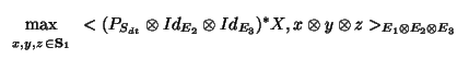
 with a linear constraint on
  as belonging to the subspace generated by the indicator matrix of
 structure
 ,
,
 . is a matrix of
  columns, each one
identifying entries of the first mode as in the current
columns, each one
identifying entries of the first mode as in the current  and
and  by a value
  ,
,  otherwise). This means that the values in will be equal for all the units with the same
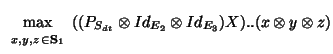
and . Writing the maximisation to find a singular value gives (denoting
otherwise). This means that the values in will be equal for all the units with the same
and . Writing the maximisation to find a singular value gives (denoting
 for
for
 ,
,
 and
and
 :
:
Equality in(15) means that PTAIV-kmodes is performed as a PTA-kmodes of
the projected data
 which in that case will be
equivalent to analyse the means data by dose and time for each band and
electrode. Note that analysing
which in that case will be
equivalent to analyse the means data by dose and time for each band and
electrode. Note that analysing
 corresponds to the residual analysis (projection on the orthogonal of the structure). Thus one has
a double decomposition of the sum of squares : explained by the structure plus its residuals, and
within each part with the SVD-modes decomposition.
Rigourously when analysing other summaries such as medians (idem for
trimean), one does not perform a PTAIV, nonetheless defining a structure by putting a
only for the median point (for each dose and time), which depends on the band
and electrode (the structure is on the whole tensor space, would provide a PTA on a
projected data.
corresponds to the residual analysis (projection on the orthogonal of the structure). Thus one has
a double decomposition of the sum of squares : explained by the structure plus its residuals, and
within each part with the SVD-modes decomposition.
Rigourously when analysing other summaries such as medians (idem for
trimean), one does not perform a PTAIV, nonetheless defining a structure by putting a
only for the median point (for each dose and time), which depends on the band
and electrode (the structure is on the whole tensor space, would provide a PTA on a
projected data.
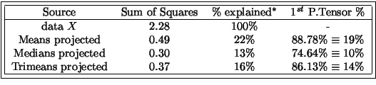
Table 3:
PTAIV Variability explained for different summaries of .
( rounded; last column: % relatively to the corresponding source
  %relatively to the
original (data ).)
%relatively to the
original (data ).)
|
|
Comparisons versus baseline for time mode and comparison versus placebo for
dose mode (the modes have been understood that way all through), are in fact already
preprocessed summary measures and can be seen as projected data. It is likely that when
performing pharmaco-EEG experiments, designs contain two baselines as in the methodology described
in introduction. Apparently the second baseline is usually taken as the reference in statistical
analysis: a greater stability is often observed with this measure(less subject variability). So
far in this paper the analysis has been done versus first baseline (08h00), and further
analysis will be done versus second baseline (08h30), the injection was in fact done at
09h00. In all the previous analysis the second baseline (versus the first) was in fact
included in the analysis, this means a true post dosing time is to be decreased by one in
the graphics.The only interest of including a (second) baseline in the analysis is when
studying the possible initial drop of activity just after injection. Nonetheless to
achieve less random subject effect, and a better comparison with reported results, thee foregoing
analysis will be done with the second baseline. It is reassuring that similar results were
obtained concerning the peak time activity but closer results, to the officially reported ones,
concerning the dose dependent band favoured for the total band effect seen the
mean analysis with nonetheless  as much important. These results were also
confirmed by a PTA-
as much important. These results were also
confirmed by a PTA- modes analysis, seen on fig.6.
Figure:
PTA-modes levels-modified data (see page.![[*]](crossref.gif) ) for all bands
(absolute energy) for verum versus placebo versus second baseline : 1
Principal Tensor.
) for all bands
(absolute energy) for verum versus placebo versus second baseline : 1
Principal Tensor.
|
|
Notice the importance of this second baseline choice towards the dose effect seen on
fig.7 and fig.6 not observed with the first baseline on the same
analysis (c.f. fig.5 fig.4(d)). The band components are quite
different as well pointing now the redistribution but also . One could see a
gradient in the slow waves and after the fast waves, but (mid-range) is now out of
pattern in these first Principal Tensors and as matter of fact does not contribute to this
Principal Tensor. The spatial components are very similar but seem more central with the analysis
versus second baseline.
Figure 7:
Same as for figure 5 but versus second baseline : 1 Principal Tensors.
|
|
Subsections
Next: Supplementary points
Up: tr00dl2
Previous: Preprocessing before a PTA-modes
Didier Leibovici
2001-09-04
![\includegraphics[width=3cm]{sy_m.ps}](img158.gif)
![\includegraphics[width=4cm]{sz_m.ps}](img159.gif)
![\includegraphics[width=6cm]{sx_m.ps}](img160.gif)
![\includegraphics[width=3cm]{sy_e.ps}](img161.gif)
![\includegraphics[width=4cm]{sz_e.ps}](img162.gif)
![\includegraphics[width=6cm]{sx_e.ps}](img163.gif)
![\includegraphics[width=3cm]{sy_t.ps}](img164.gif)
![\includegraphics[width=4cm]{sz_t.ps}](img165.gif)
![\includegraphics[width=6cm]{sx_t.ps}](img166.gif)
![\includegraphics[width=3cm]{cymea.ps}](img196.gif)
![\includegraphics[width=4cm]{czmea.ps}](img197.gif)
![\includegraphics[width=6cm]{cxmea.ps}](img198.gif)
![\includegraphics[width=3cm]{cymed.ps}](img199.gif)
![\includegraphics[width=4cm]{czmed.ps}](img200.gif)
![\includegraphics[width=6cm]{cxmed.ps}](img201.gif)
![\includegraphics[width=3cm]{cytri.ps}](img202.gif)
![\includegraphics[width=4cm]{cztri.ps}](img203.gif)
![\includegraphics[width=6cm]{cxtri.ps}](img204.gif)